A Simplified Path Diagram for the Spleen Data
The main simplification in the path diagram is to drop all the error terms in the model. Instead, error variances are treated as residual (or partial) variances for the endogenous variables in the model or path diagram. Hence, in the path diagrams for RAM models, error variances are also represented by double-headed arrows directly attached to the endogenous variables, which is the same way you represent variances for the exogenous variables. The RAM model convention leads to a simplified representation of the path diagram for the spleen data, as shown in Figure 17.14.
Figure 17.14: Simplified Path Diagram: Spleen
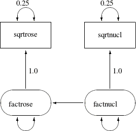
Another simplification done in Figure 17.14 is the omission of the parameter labeling in the path diagram. This simplification is not a part of the RAM notation. It
is just a convention in PROC CALIS that you can omit the unconstrained parameter names without affecting the meaning of the
model. Hence, the parameter names beta, v_disturb, and v_factnucl are no longer necessary in the simplified path diagram Figure 17.14. As you can see, this convention makes the task of model specification considerably simpler and easier.
The following statements show the specification of the simplified path diagram in Figure 17.14:
proc calis data=spleen;
   path
      sqrtrose <=== factrose   = 1.0,
      sqrtnucl <=== factnucl   = 1.0,
      factrose <=== factnucl   ;
   pvar
      sqrtrose = 0.25,      /* error variance for sqrtrose */
      sqrtnucl = 0.25,      /* error variance for sqrtnucl */
      factrose,             /* disturbance/error variance for factrose */
      factnucl;             /* variance of factnucl */
run;
The PATH statement invokes the PATH modeling language of PROC CALIS. In the PATH modeling language, each entry of specification corresponds to either a single- or double- headed arrow specification in the path diagram shown in Figure 17.14, as explained in the following:
-
The PATH statement enables you to specify each of the single-headed arrows (paths) as path entries, which are separated by commas. You have three single-headed arrows in the path diagram and therefore you have three path entries in the PATH statement. The path entries “
sqrtrose <=== factrose” and “sqrtnucl <=== factnucl” are followed by the constant 1, indicating fixed path coefficients. The path “factrose <=== factnucl” is also specified, but without giving a fixed value or a parameter name. By default, this path entry is associated with a free parameter for the effect or path coefficient. -
The PVAR statement enables you to specify each of the double-headed arrows with both heads pointing to the same variable, exogenous or endogenous. This type of arrows represents variances or error variances. You have four such double-headed arrows in the path diagram, and therefore there are four corresponding entries under the PVAR statement. Two of them are assigned with fixed constants (0.25), and the remaining two (error variance of
factroseand variance offactnucl) are free variance parameters. -
The PCOV statement enables you to specify each of the double-headed arrows with its heads pointing to different variables, exogenous or endogenous. This type of arrows represents covariances between variables or their error terms. You do not have this type of double-headed arrows in the current path diagram, and therefore you do not need a PCOV statement for the corresponding model specification.
The estimation results are shown in Figure 17.15. Essentially, these are exactly the same estimation results as those that result from the LINEQS modeling language for the just-identified model in section Illustration of Model Identification: Spleen Data.
Figure 17.15: Spleen Data: RAM Model
| PATH List | ||||||
|---|---|---|---|---|---|---|
| Path | Parameter | Estimate | Standard Error |
t Value | ||
| sqrtrose | <=== | factrose | 1.00000 | |||
| sqrtnucl | <=== | factnucl | 1.00000 | |||
| factrose | <=== | factnucl | _Parm1 | 0.39074 | 0.07708 | 5.06920 |
| Variance Parameters | |||||
|---|---|---|---|---|---|
| Variance Type |
Variable | Parameter | Estimate | Standard Error |
t Value |
| Error | sqrtrose | 0.25000 | |||
| sqrtnucl | 0.25000 | ||||
| factrose | _Parm2 | 0.38153 | 0.28556 | 1.33607 | |
| Exogenous | factnucl | _Parm3 | 10.50458 | 4.58577 | 2.29069 |
Notice in Figure 17.15 that the path coefficient for path “factrose <=== factnucl” is given a parameter name _Parm1, which is generated automatically by PROC CALIS. This is the same beta parameter of the LINEQS model in the section Illustration of Model Identification: Spleen Data. Also, the variance parameters _Parm2 and _Parm3 in Figure 17.15 are the same v_disturb and v_factnucl parameters, respectively, in the preceding LINEQS model.
In PROC CALIS, using parameter names to specify free parameters is optional. Parameter names are generated for free parameters by default. Or, if you choose parameter names for your own convenience, you can do so without changing the model specification. For example, you can specify the preceding PATH model equivalently by adding the desired parameter names, as shown in the following statements:
proc calis data=spleen;
   path
      sqrtrose <=== factrose   = 1.0,
      sqrtnucl <=== factnucl   = 1.0,
      factrose <=== factnucl   = beta;
   pvar
      sqrtrose = 0.25,       /* error variance for sqrtrose */
      sqrtnucl = 0.25,       /* error variance for sqrtnucl */
      factrose = v_disturb,  /* disturbance/error variance for factrose */
      factnucl = v_factnucl; /* variance of factnucl */
run;
A path diagram provides you an easy and conceptual way to represent your model, while the PATH modeling language in PROC CALIS offers you an easy way to input your path diagram in a non-graphical fashion. This is especially useful for models with more complicated path structures. See the section A Combined Measurement-Structural Model for a more elaborated example of the PATH model application.
The next section provides examples of the PATH model applied to classical test theory.