The Example
Suppose you want to compare survival rates for an existing cancer treatment and a new treatment. You intend to use a log-rank test to compare the overall survival curves for the two treatments. You want to determine a sample size to achieve a power of 0.8 for a two-sided test using a balanced design, with a significance level of 0.05.
The survival curve of patients for the existing treatment is known to be approximately exponential with a median survival time of five years. You think that the proposed treatment will yield a survival curve described by the times and probabilities listed in Table 72.9. Patients are to be accrued uniformly over two years and followed for three years.
Table 72.9: Survival Probabilities for Proposed Treatment
|
Time |
Probability |
|---|---|
|
1 |
0.95 |
|
2 |
0.90 |
|
3 |
0.75 |
|
4 |
0.70 |
|
5 |
0.60 |
To create a new survival analysis project, select →, Then, under the Survival Analysis section, select and click . The project appears with the Edit Properties page displayed.
Editing Properties
Project Description
For the example, change the project description to Comparing cancer treatments using two-sample survival rank test.
Figure 72.78: Project Description and Solve For Tab
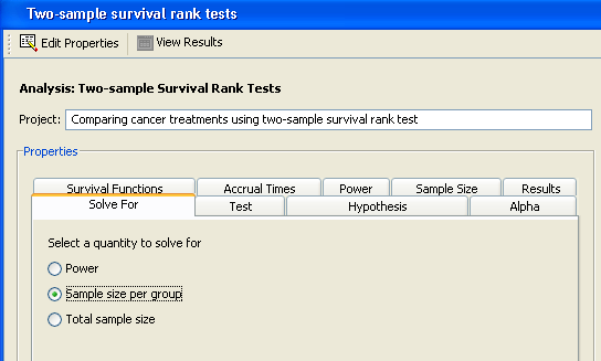
Solve For
Click the Solve For tab to select the quantity to solve for. For this example, select the option, as shown in Figure 72.78. For information about calculating total sample size, see the section Solving for Sample Size.
In this analysis you can solve for power, sample size per group, or total sample size.
Test
Click the Test tab to select a rank test. For this example, select the option, as shown in Figure 72.79.
Figure 72.79: Test Tab
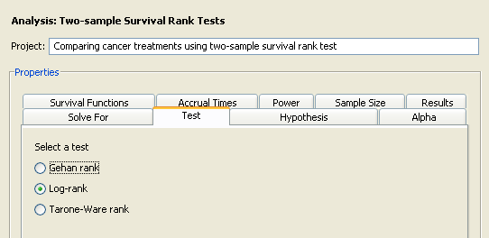
Several rank tests are available: Gehan, log-rank, and Tarone-Ware. The Gehan test is most sensitive to survival differences near the beginning of the study period, the log-rank test is uniformly sensitive throughout the study period, and the Tarone-Ware test is somewhere in between.
Hypothesis
Click the Hypothesis tab to select a one- or two-sided test. For the example, select the option, as shown in Figure 72.80.
Figure 72.80: Hypothesis Tab
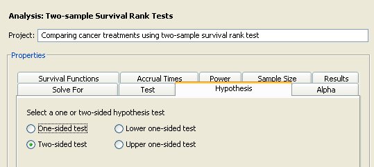
You can choose either a one- or two-sided test. For the one-sided test, the alternative hypothesis is assumed to be in the same direction as the effect. If you do not know the direction of the effect (that is, whether it is positive or negative), the two-sided test is appropriate. If you know the effect’s direction, the one-sided test is appropriate. If you specify a one-sided test and the effect is in the unexpected direction, the results of the analysis are invalid.
Alpha
Click the Alpha tab to enter one or more values for the significance level. For the example, enter the desired significance level of 0.05 in the first cell of the Alpha table, as shown in Figure 72.81, if it is not already the default value.
Figure 72.81: Alpha Tab
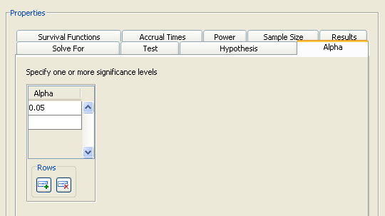
The significance level is the probability of falsely rejecting the null hypothesis. If you frequently use the same values for alpha, set them as the defaults in the Preferences window.
Survival Functions
Click the Survival Functions tab to select the input form for the survival functions.
Figure 72.82: Survival Functions Tab with Number of Curves
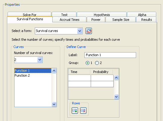
Examine the input alternatives available in the Select a form list. There are four alternate forms for entering survival functions. The first three apply only to exponential curves; the fourth applies to both piecewise linear and exponential curves.
-
Enter median survival times for the two groups.
-
Enter hazards for the two groups.
-
Enter hazards for the reference group and hazard ratios.
-
Enter survival probabilities and their associated times for each of several curves. Select or enter the number of curves from the drop-down list; at least two curves are required. Then, for each curve, select it in the left-hand list, select the Group 1 or Group 2 option, and then define the survival curve by entering pairs of times and probabilities. Enter a time and probability pair only if the probability is less than that of the previous pair.
For information about using the other forms, see the section Using the Other Survival Curve Forms.
For each survival curve, select the curve in the left-hand list. Then, enter a descriptive label and select which group it is for. The labels should be unique. Finally, enter pairs of survival times and probabilities.
When you enter probabilities, enter a time and probability pair only when the probability for a survival curve changes. For example, if the probability for curve 1 at time 1 and 2 is 0.9 and at time 3 is 0.8, enter 0.9 for time 1 and 0.8 for time 3.
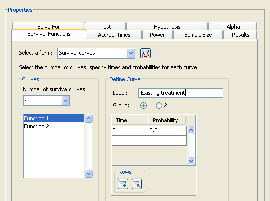
To specify an exponential survival curve, enter a single time and probability pair. In the example, the exponential curve for the existing treatment is defined by a probability of 0.5 at time 5.
The units of time for the survival curves must correspond to the units for the accrual, follow-up, and total times, which are described in the section Accrual Times.
You can also compare several survival curves. For example, if you have two scenarios, A and B, for group 1’s curve and two scenarios, C and D, for group 2’s curve, then specify probabilities for the four curves and assign A and B to group 1 and C and D to group 2.
For the example, select the form, as shown in Figure 72.82. Enter the value, 2, in the Number of survival curves list box.
For the example enter the following values:
-
For the first survival curve, enter a label of
Existing treatmentand select the option. For the first curve, enter a time of 5 and a probability of 0.5. Figure 72.83 shows the resulting values.Figure 72.83: Survival Times and Probabilities for Curve 1
-
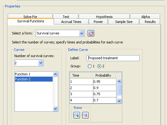
For the second curve select
Function 2in the selection list on the left side of the tab. Enter a label ofProposed treatmentand select the option. Then, enter time values of 1 through 5 and the corresponding probabilities of 0.95, 0.9, 0.75, 0.7, and 0.6. To add rows to the table, click the button beneath the table.
Figure 72.84 shows these values; the last row of the time and probability table is not displayed.
Figure 72.84: Survival Times and Probabilities for Curve 2
Accrual Times
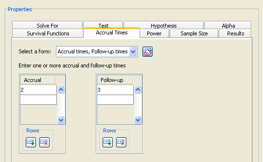
Click the Accrual times tab to select an input form for accrual times and to enter the times.
Figure 72.85: Accrual Times Tab
Examine the alternatives available in the Select a form list.
Accrual time is the period during which subjects are brought into the study. Follow-up time is the period during which subjects are observed after all subjects have been included in the study. Total time is the sum of accrual and follow-up time. The units of time for the accrual, follow-up, and total times must correspond to the units you used specified for the survival curves.
When you enter survival curves, the sum of the accrual and follow-up times must be less than the largest time for each survival curve. This does not apply to survival curves represented by a single time, which represent exponential curves.
On the Accrual Times tab, there are three alternate forms for entering accrual and follow-up times:
-
Enter accrual and follow-up times.
-
Enter accrual and total times.
-
Enter follow-up and total times.
For the example, select the form. Then enter a single value of 2 in the Accrual table and a value of 3 in the Follow-up table, as shown in Figure 72.85.
Power
Click the Power tab to enter one or more power values. For the example, enter a single value of 0.8.
When you calculate sample size, it is necessary to specify one or more powers.
Summary of Input Parameters
Table 72.10 contains the values of the input parameters for the example.
Table 72.10: Summary of Input Parameters
|
Parameter |
Value |
|---|---|
|
Solve for |
Sample size per group |
|
Test |
Log-rank |
|
Hypothesis |
Two-sided test |
|
Alpha |
0.05 |
|
Survival function form |
Survival curves |
|
Survival curves |
See Table 72.11 and Table 72.12 |
|
Accrual and follow-up times form |
Accrual time, Follow-up times |
|
Accrual times |
2 |
|
Follow-up times |
3 |
|
Power |
0.8 |
Table 72.11 and Table 72.12 contain times and probabilities for the two survival curves, respectively.
Table 72.11: Survival Times and Probabilities for Existing Treatment (Survival Curve 1)
|
Time |
Probability |
|---|---|
|
5 |
0.5 |
Table 72.12: Survival Times and Probabilities for Proposed Treatment (Survival Curve 2)
|
Time |
Probability |
|---|---|
|
1 |
0.95 |
|
2 |
0.90 |
|
3 |
0.75 |
|
4 |
0.70 |
|
5 |
0.60 |
Result Options
Click the Results tab to specify the desired result options. For the example, request both results by selecting both the and check boxes.
Specifying only one power (as in this example) produces a graph with a single point. You might be interested in a plot of sample sizes for a range of powers—say, between 0.75 and 0.85. You can customize the graph by specifying the values for the power axis. Also, you might want to change the appearance of the graph to have sample size (per group) on the vertical axis and power on the horizontal axis.
Click the button beside the check box to customize the graph. The Customize Graph window is displayed, as shown in Figure 72.86.
Figure 72.86: Customize Graph Window with Axis Orientation Tab
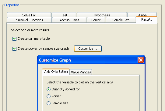
Click the Axis Orientation tab to select which variable to plot on the vertical axis. For the example, select the option, as shown in Figure 72.86. This option plots sample size on the vertical axis and power on the horizontal axis. You could also have chosen the option.
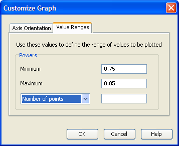
Click the Value Ranges tab to enter minimum and maximum values for a plot axis. For the example, enter a minimum of 0.75 and a maximum of 0.85 in the Powers text boxes. This sets the range of values on the axis for powers. The completed Value Ranges tab of the window
is displayed in Figure 72.87. You can set the axis values only for the quantity that is not being solved for.
Figure 72.87: Customize Graph Window with Value Ranges Tab
Click to save the values that you have entered and return to the Edit Properties page.
Then, click to perform the analysis. If there are no errors in the input parameter values, the View Results page appears. If there are errors in the input parameter values, you are prompted to correct them.
Viewing Results
The results appear in separate tabs on the View Results page of the project. Select the tab of each result that you want to view.
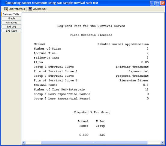
Summary Table
Click the Summary Table tab to view the summary table. It is composed of two subtables. As shown in Figure 72.88, the Fixed Scenario Elements and Computed N Per Group tables include the values of the input parameters and the computed quantity (in this case, sample size per group, N per group). The sample size per group for the single requested scenario is 226.
Figure 72.88: Summary Table
Power by Sample Size Graph
Click the Graph tab to view the power by sample size graph.
Figure 72.89: Power by Sample Size Graph
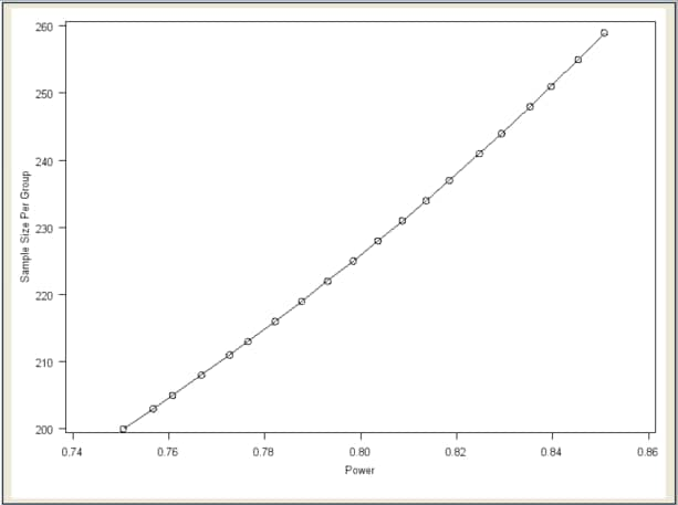
As you can see in Figure 72.89, the graph is curved slightly upward with larger powers associated with larger sample sizes. Sample size is plotted on the vertical axis as requested in the Customize Graph window.
Narratives
Click the Narratives tab to create one or more narratives. To generate a narrative, select the single scenario in the narrative selector table at the bottom of the tab. The narrative for this task does not include the survival times and probabilities for the survival curves:
For a log-rank test comparing two survival curves with a two-sided significance level of 0.05, assuming uniform accrual with an accrual time of 2 and a follow-up time of 3, a sample size of 226 per group is required to obtain a power of at least 0.8 for the exponential curve, “Existing treatment,” and the piecewise linear curve, “Proposed treatment.” The actual power is 0.800.
For information about selecting additional narratives when multiple scenarios are present, see the section Creating Narratives.