The Example
Suppose you are interested in testing how two experimental drugs affect systolic blood pressure relative to a standard drug. You want to include both men and women in the study. You have a two-factor design: a drug factor with three levels and a gender factor with two levels. You choose a main-effects-only model because you do not expect a drug by gender interaction. You want to calculate the sample size that will produce a power of 0.9 using a significance level of 0.05. You believe that the error standard deviation is between 5 and 7 mm pressure. This is a two-way analysis of variance, so the general linear univariate models task is the appropriate one.
Editing Properties
Start by opening the New window (→). In the Analysis of Variance and Linear models section of the New window, select . The project appears, with the Edit Properties page displayed.
Project Description
For the example, change the project description to Three blood pressure drugs and gender.
Variables
Click the Variables tab to enter the names of the factors in the design. Click the button. The Factor Definition window appears, as shown in Figure 72.60.
Figure 72.60: Factor Definition Window
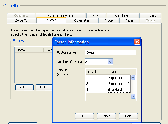
Enter the name for the first factor, Drug, and enter the number of factor levels in the Number of levels: list box. There are three levels for this factor. Optionally, you can provide a label for each factor level. This label is
used to identify factor levels on other tabs of the Edit Properties page. For this example enter the labels Experimental 1, Experimental 2, and Standard for the three levels of the Drug factor. Click when you are finished.
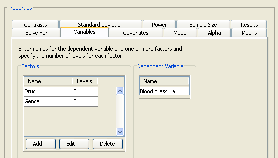
Click the button again and repeat the process for the second factor, Gender with two levels and labels Female and Male.
Factors can contain blanks and other special characters. Do not use an asterisk (*) because a factor name with an asterisk might be confused with an interaction effect. Factor names can be any length, but they must be distinct from one another in the first 32 characters.
On the Variables tab, you can also specify the name of the dependent variable; in this example, Blood pressure is used.
The completed Variables tab is shown in Figure 72.61.
Figure 72.61: Variables Tab with Factors and Number of Levels
Model
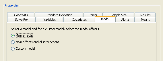
Click the Model tab, then choose from three model options:
-
Only the main effects are included in the model.
-
The main effects and all possible interactions are included in the model.
-
Selected effects are included in the model. The effects are selected in a model builder that is displayed when this model is selected. For more information about specifying a custom model, see the section Specifying a Custom Model.
For this example, choose the default model, as shown in Figure 72.62.
Figure 72.62: Model Tab with Main Effects Selected
Alpha
Click the Alpha tab to specify one or more significance levels. For the example, specify a single significance level of 0.05.
Alpha is the significance level (that is, the probability of falsely rejecting the null hypothesis). If you frequently use the same values for alpha, set them as the defaults in the Preferences window (→).
Means
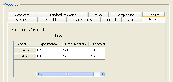
Click the Means tab to enter projected cell means for each cell of the design. The completed means for the example are shown in Figure 72.63.
Figure 72.63: Means Tab with Cell Means
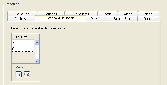
Standard Deviation
Click the Standard Deviation tab to specify one or more conjectured error standard deviations. The standard deviation is the same as the root mean squared error. For this example, enter two standard deviations, 5 and 7, as shown in Figure 72.64.
Figure 72.64: Standard Deviations Tab
Relative Sample Size
Click the Sample Size tab to select whether cell sample sizes are equal or unequal.
Figure 72.65: Sample Size Tab with Equal Cell Sample Sizes
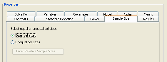
For the example, select the option, as shown in Figure 72.65.
When solving for sample size, it is necessary to specify whether the cell sample sizes are equal or unequal. If cell sizes are unequal, relative sample size weights must also be specified. For more information about providing sample size weights, see the section Using Unequal Cell Sizes.
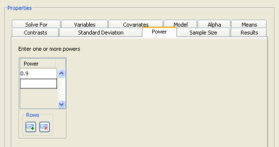
Power
Click the Power tab to specify one or more powers. For this example, enter a single power of 0.9, as shown in Figure 72.66.
Figure 72.66: Power Tab
Summary of Input Parameters
Table 72.6 contains the values of the input parameters for the example.
Table 72.6: Summary of Input Parameters
|
Parameter |
Value |
|---|---|
|
Model |
Main effects |
|
Alpha |
0.05 |
|
Means |
See Table 72.7 |
|
Standard deviation |
5, 7 |
|
Relative sample sizes |
Equal cell sizes |
|
Power |
0.9 |
Table 72.7: Cell Means
|
Drug |
|||
|---|---|---|---|
|
Gender |
Experimental 1 |
Experimental 2 |
Standard |
|
Female |
125 |
121 |
118 |
|
Male |
130 |
128 |
125 |
Results Options
Click the Results tab to select desired results. For the example, select both the and check boxes.
The graph consists of four points, one for each of the four scenarios that were created by combining the two factor main effects with the two standard deviations. This graph is not very informative, so specify a range of powers for the horizontal power axis. To change the power axis of the graph, click the button beside the check box to open the Customize Graph window.
Figure 72.67: Value Ranges on Customize Graph Window
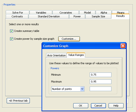
Click the Value Ranges tab and enter a minimum power of 0.75 and a maximum power of 0.95, as shown in Figure 72.67. Click to close the window.
Now, click to perform the analysis.
Viewing Results
The results are displayed in separate tabs on the View Results page.
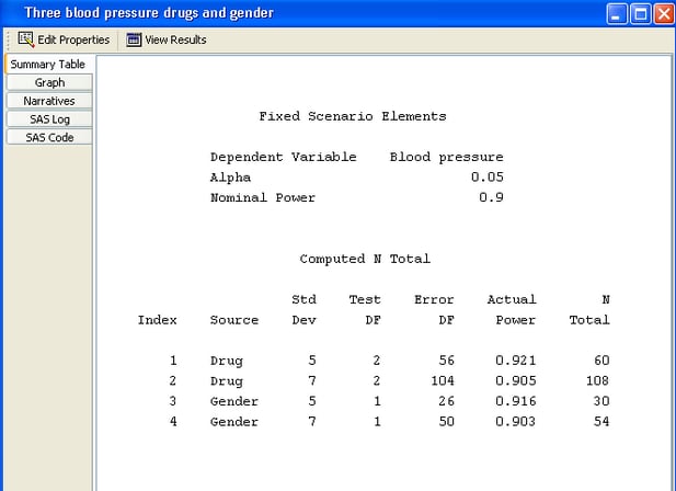
Click the Summary Table tab to view the summary table. In the Computed N Total table, sample sizes are listed for each combination of factor and standard deviation (Figure 72.68). You need a total sample size between 60 and 108 to yield a power of 0.9 for the Drug effect if the standard deviation is between 5 and 7. You need a sample size of half that for the Gender effect.
Figure 72.68: Summary Table
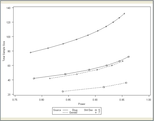
Click the Graph tab to view the power by sample size graph, as shown in Figure 72.69. One approximately linear curve is displayed for each standard deviation and factor combination.
Figure 72.69: Power by Sample Size Graph
Click the Narratives tab to create narratives of one or more scenarios. Select the first scenario, the Drug effect with the standard deviation of 5, in the narrative selector table. Note that the cell means are not included in the following narrative description:
For the usual F test of the Drug effect in the general linear univariate model with fixed class effects [Blood pressure =
                           Drug Gender] using a significance level of 0.05, assuming the specified cell means and an error standard deviation of 5, a
                           total sample size of 60 assuming a balanced design is required to obtain a power of at least 0.9. The actual power is 0.921.
For more information about using the narrative facility, see the section Creating Narratives.