The ACECLUS Procedure

Example 23.1 Transformation and Cluster Analysis of Fisher Iris Data
The iris data published by Fisher (1936) have been widely used for examples in discriminant analysis and cluster analysis. The sepal length, sepal width, petal length, and petal width are measured in millimeters on 50 iris specimens from each of three species, Iris setosa, I. versicolor, and I. virginica. Mezzich and Solomon (1980) discuss a variety of cluster analyses of the iris data.
In this example PROC ACECLUS is used to transform the iris data, which is available from the Sashelp library, and the clustering is performed by PROC FASTCLUS. Compare this with the example in Chapter 36: The FASTCLUS Procedure. The results from the FREQ procedure display fewer misclassifications when PROC ACECLUS is used.
The following statements produce Output 23.1.1 through Output 23.1.5:
title 'Fisher (1936) Iris Data';

proc aceclus data=sashelp.iris out=ace p=.02 outstat=score;
   var SepalLength SepalWidth PetalLength PetalWidth ;
run;
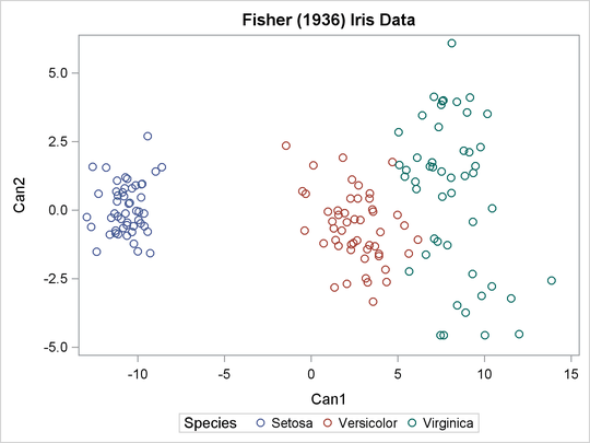
proc sgplot data=ace;
   scatter y=can2 x=can1 / group=Species;
   keylegend / title="Species";
run;
proc fastclus data=ace maxc=3 maxiter=10 conv=0 out=clus;
   var can:;
run;
proc freq;
   tables cluster*Species;
run;
Output 23.1.1: Using PROC ACECLUS to Transform Fisher’s Iris Data
| Fisher (1936) Iris Data |
| Observations | 150 | Proportion | 0.0200 |
|---|---|---|---|
| Variables | 4 | Converge | 0.00100 |
| Means and Standard Deviations | |||
|---|---|---|---|
| Variable | Mean | Standard Deviation |
Label |
| SepalLength | 58.4333 | 8.2807 | Sepal Length (mm) |
| SepalWidth | 30.5733 | 4.3587 | Sepal Width (mm) |
| PetalLength | 37.5800 | 17.6530 | Petal Length (mm) |
| PetalWidth | 11.9933 | 7.6224 | Petal Width (mm) |
| COV: Total Sample Covariances | ||||
|---|---|---|---|---|
| SepalLength | SepalWidth | PetalLength | PetalWidth | |
| SepalLength | 68.5693512 | -4.2434004 | 127.4315436 | 51.6270694 |
| SepalWidth | -4.2434004 | 18.9979418 | -32.9656376 | -12.1639374 |
| PetalLength | 127.4315436 | -32.9656376 | 311.6277852 | 129.5609396 |
| PetalWidth | 51.6270694 | -12.1639374 | 129.5609396 | 58.1006264 |
| Threshold = | 0.334211 |
|---|
| Iteration History | ||||
|---|---|---|---|---|
| Iteration | RMS Distance |
Distance Cutoff |
Pairs Within Cutoff |
Convergence Measure |
| 1 | 2.828 | 0.945 | 408.0 | 0.465775 |
| 2 | 11.905 | 3.979 | 559.0 | 0.013487 |
| 3 | 13.152 | 4.396 | 940.0 | 0.029499 |
| 4 | 13.439 | 4.491 | 1506.0 | 0.046846 |
| 5 | 13.271 | 4.435 | 2036.0 | 0.046859 |
| 6 | 12.591 | 4.208 | 2285.0 | 0.025027 |
| 7 | 12.199 | 4.077 | 2366.0 | 0.009559 |
| 8 | 12.121 | 4.051 | 2402.0 | 0.003895 |
| 9 | 12.064 | 4.032 | 2417.0 | 0.002051 |
| 10 | 12.047 | 4.026 | 2429.0 | 0.000971 |
| Algorithm converged. |
Output 23.1.2: Eigenvalues, Raw Canonical Coefficients, and Standardized Canonical Coefficients
| ACE: Approximate Covariance Estimate Within Clusters | ||||
|---|---|---|---|---|
| SepalLength | SepalWidth | PetalLength | PetalWidth | |
| SepalLength | 11.73342939 | 5.47550432 | 4.95389049 | 2.02902429 |
| SepalWidth | 5.47550432 | 6.91992590 | 2.42177851 | 1.74125154 |
| PetalLength | 4.95389049 | 2.42177851 | 6.53746398 | 2.35302594 |
| PetalWidth | 2.02902429 | 1.74125154 | 2.35302594 | 2.05166735 |
| Eigenvalues of Inv(ACE)*(COV-ACE) | ||||
|---|---|---|---|---|
| Eigenvalue | Difference | Proportion | Cumulative | |
| 1 | 63.7716 | 61.1593 | 0.9367 | 0.9367 |
| 2 | 2.6123 | 1.5561 | 0.0384 | 0.9751 |
| 3 | 1.0562 | 0.4167 | 0.0155 | 0.9906 |
| 4 | 0.6395 | 0.00939 | 1.0000 | |
| Eigenvectors (Raw Canonical Coefficients) | |||||
|---|---|---|---|---|---|
| Can1 | Can2 | Can3 | Can4 | ||
| SepalLength | Sepal Length (mm) | -.012009 | -.098074 | -.059852 | 0.402352 |
| SepalWidth | Sepal Width (mm) | -.211068 | -.000072 | 0.402391 | -.225993 |
| PetalLength | Petal Length (mm) | 0.324705 | -.328583 | 0.110383 | -.321069 |
| PetalWidth | Petal Width (mm) | 0.266239 | 0.870434 | -.085215 | 0.320286 |
| Standardized Canonical Coefficients | |||||
|---|---|---|---|---|---|
| Can1 | Can2 | Can3 | Can4 | ||
| SepalLength | Sepal Length (mm) | -0.09944 | -0.81211 | -0.49562 | 3.33174 |
| SepalWidth | Sepal Width (mm) | -0.91998 | -0.00031 | 1.75389 | -0.98503 |
| PetalLength | Petal Length (mm) | 5.73200 | -5.80047 | 1.94859 | -5.66782 |
| PetalWidth | Petal Width (mm) | 2.02937 | 6.63478 | -0.64954 | 2.44134 |
Output 23.1.3: Plot of Transformed Iris Data: PROC SGPLOT
Output 23.1.4: Clustering of Transformed Iris Data: Partial Output from PROC FASTCLUS
| Fisher (1936) Iris Data |
| Cluster Summary | ||||||
|---|---|---|---|---|---|---|
| Cluster | Frequency | RMS Std Deviation | Maximum Distance from Seed to Observation |
Radius Exceeded |
Nearest Cluster | Distance Between Cluster Centroids |
| 1 | 50 | 1.4138 | 5.3152 | 2 | 5.8580 | |
| 2 | 50 | 1.8880 | 6.8298 | 1 | 5.8580 | |
| 3 | 50 | 1.1016 | 5.2768 | 1 | 13.2845 | |
| Statistics for Variables | ||||
|---|---|---|---|---|
| Variable | Total STD | Within STD | R-Square | RSQ/(1-RSQ) |
| Can1 | 8.04808 | 1.48537 | 0.966394 | 28.756658 |
| Can2 | 1.90061 | 1.85646 | 0.058725 | 0.062389 |
| Can3 | 1.43395 | 1.32518 | 0.157417 | 0.186826 |
| Can4 | 1.28044 | 1.27550 | 0.021025 | 0.021477 |
| OVER-ALL | 4.24499 | 1.50298 | 0.876324 | 7.085666 |
| Pseudo F Statistic = | 520.80 |
|---|
| Approximate Expected Over-All R-Squared = | 0.80391 |
|---|
| Cubic Clustering Criterion = | 5.179 |
|---|
| Cluster Means | ||||
|---|---|---|---|---|
| Cluster | Can1 | Can2 | Can3 | Can4 |
| 1 | 2.54528754 | -0.59273569 | -0.78905317 | -0.26079612 |
| 2 | 8.12988211 | 0.52566663 | 0.51836499 | 0.14915404 |
| 3 | -10.67516964 | 0.06706906 | 0.27068819 | 0.11164209 |
| Cluster Standard Deviations | ||||
|---|---|---|---|---|
| Cluster | Can1 | Can2 | Can3 | Can4 |
| 1 | 1.572366584 | 1.393565864 | 1.303411851 | 1.372050319 |
| 2 | 1.799159552 | 2.743869556 | 1.270344142 | 1.370523175 |
| 3 | 0.953761025 | 0.931943571 | 1.398456061 | 1.058217627 |
Output 23.1.5: Crosstabulation of Cluster by Species for Fisher’s Iris Data: PROC FREQ
| Fisher (1936) Iris Data |
|
|
|||||||||||||||||||||||||||||||||||||||||||||||||||||||||||||||||||||||||||||||||||||||||||||||