PROC TTEST: One-Sample Comparison with the FREQ Statement

Example 95.2 One-Sample Comparison with the FREQ Statement

This example examines children’s reading skills. The data consist of Degree of Reading Power (DRP) test scores from 44 third-grade children and are taken from Moore (1995, p. 337). Their scores are given in the following DATA step:

data read;
   input score count @@;
   datalines;
40 2   47 2   52 2   26 1   19 2
25 2   35 4   39 1   26 1   48 1
14 2   22 1   42 1   34 2   33 2
18 1   15 1   29 1   41 2   44 1
51 1   43 1   27 2   46 2   28 1
49 1   31 1   28 1   54 1   45 1
;
run;

The following statements invoke the TTEST procedure to test if the mean test score is equal to 30.

ods graphics on;

proc ttest data=read h0=30;
   var score;
   freq count;
run;

ods graphics off;

The count variable contains the frequency of occurrence of each test score; this is specified in the FREQ statement. The output, shown in Output 95.2.1, contains the results.

Output 95.2.1 TTEST Results

The TTEST Procedure

Variable: score

N	Mean	Std Dev	Std Err	Minimum	Maximum
44	34.8636	11.2303	1.6930	14.0000	54.0000

Mean	95% CL Mean		Std Dev	95% CL Std Dev
34.8636	31.4493	38.2780	11.2303	9.2788	14.2291

DF	t Value	Pr > \|t\|
43	2.87	0.0063

The SAS log states that 30 observations and two variables have been read. However, the sample size given in the TTEST output is N=44. This is due to specifying the count variable in the FREQ statement. The test is significant $\text{[math]}$ , $\text{[math]}$ at the 5% level, so you can conclude that the mean test score is different from 30.

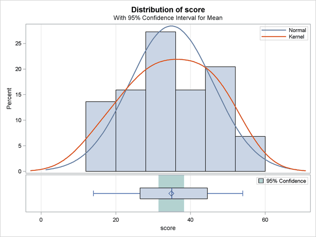
The summary panel in Output 95.2.2 shows a histogram with overlaid normal and kernel densities, a box plot, and the 95% confidence interval for the mean.

Output 95.2.2 Summary Panel

The Q-Q plot in Output 95.2.3 assesses the normality assumption.

Output 95.2.3 Q-Q Plot

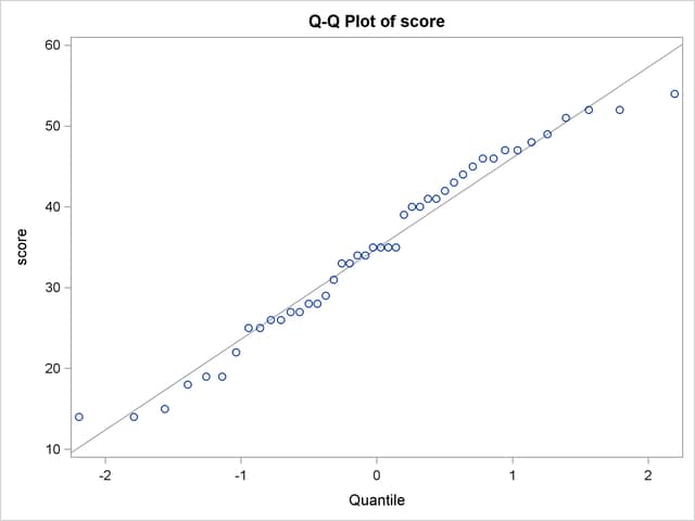
The tight clustering of the points around the diagonal line is consistent with the normality assumption. You could use the UNIVARIATE procedure with the NORMAL option to numerically check the normality assumption.