The PRINQUAL Procedure
- Overview
- Getting Started
-
Syntax

-
Details
The Three Methods of Variable Transformation Understanding How PROC PRINQUAL Works Splines Missing Values Controlling the Number of Iterations Performing a Principal Component Analysis of Transformed Data Using the MAC Method Output Data Set Avoiding Constant Transformations Constant Variables Character OPSCORE Variables REITERATE Option Usage Passive Observations Computational Resources Displayed Output ODS Table Names ODS Graphics
-
Examples
- References
Getting Started: PRINQUAL Procedure
PROC PRINQUAL can be used to fit a principal component model with nonlinear transformations of the variables and graphically display the results. This example finds monotonic transformations of ratings of automobiles.
title 'Ratings for Automobiles Manufactured in 1980';

data cars;
   input Origin $ 1-8 Make $ 10-19 Model $ 21-36
         (MPG Reliability Acceleration Braking Handling Ride
          Visibility Comfort Quiet Cargo) (1.);
   datalines;
GMC      Buick      Century         3334444544
GMC      Buick      Electra         2434453555
GMC      Buick      Lesabre         2354353545

   ... more lines ...

GMC      Pontiac    Sunbird         3134533234
;
ods graphics on;

proc prinqual data=cars plots=all maxiter=100;
   transform monotone(mpg -- cargo);
   id model;
run;
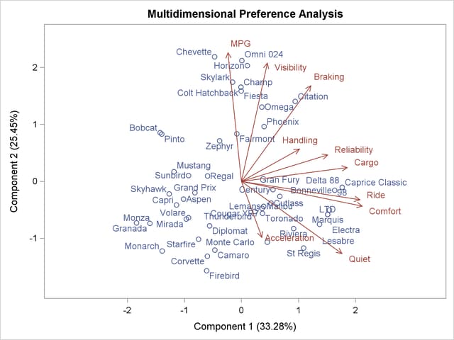
The PROC PRINQUAL statement names the input data set Cars. The ODS GRAPHICS statement, along with the PLOTS=ALL option, requests all graphical displays. The MDPREF option requests the PCA plot with the scores (automobiles) represented as points and the structure (variables) represented as vectors. By default, the vector lengths are increased by a factor of 2.5 to produce a better graphical display. If instead you were to specify MDPREF=1, you would get the actual vectors, and they would all be short and would end near the origin where there are a lot of points. It is often the case that increasing the vector lengths by a factor of 2 or 3 makes a better graphical display, so by default the vector lengths are increased by a factor of 2.5. Up to 100 iterations are requested with the MAXITER= option. All of the numeric variable are specified with a MONOTONE transformation, so their original values, 1 to 5, are optimally rescored to maximize fit to a two-component model while preserving the original order. The Model variable provides the labels for the row points in the plot.
The iteration history table is shown in Figure 73.1. The monotonic transformations allow the PCA to account for 5% more variance in two principal components than the ordinary PCA model applied to the untransformed data.
| Ratings for Automobiles Manufactured in 1980 |
| PRINQUAL MTV Algorithm Iteration History | |||||
|---|---|---|---|---|---|
| Iteration Number |
Average Change |
Maximum Change |
Proportion of Variance |
Criterion Change |
Note |
| 1 | 0.18087 | 1.24219 | 0.53742 | ||
| 2 | 0.06916 | 0.77503 | 0.57244 | 0.03502 | |
| 3 | 0.04653 | 0.38237 | 0.57978 | 0.00734 | |
| 4 | 0.03387 | 0.18682 | 0.58300 | 0.00321 | |
| 5 | 0.02661 | 0.13506 | 0.58484 | 0.00185 | |
| 6 | 0.01730 | 0.09213 | 0.58600 | 0.00115 | |
| 7 | 0.00969 | 0.07107 | 0.58660 | 0.00061 | |
| 8 | 0.00705 | 0.04798 | 0.58685 | 0.00025 | |
| 9 | 0.00544 | 0.03482 | 0.58699 | 0.00014 | |
| 10 | 0.00442 | 0.02641 | 0.58708 | 0.00009 | |
| 11 | 0.00363 | 0.02062 | 0.58714 | 0.00006 | |
| 12 | 0.00298 | 0.01643 | 0.58717 | 0.00004 | |
| 13 | 0.00245 | 0.01325 | 0.58720 | 0.00002 | |
| 14 | 0.00201 | 0.01077 | 0.58721 | 0.00002 | |
| 15 | 0.00165 | 0.00880 | 0.58723 | 0.00001 | |
| 16 | 0.00136 | 0.00721 | 0.58723 | 0.00001 | |
| 17 | 0.00112 | 0.00591 | 0.58724 | 0.00001 | |
| 18 | 0.00092 | 0.00485 | 0.58724 | 0.00000 | |
| 19 | 0.00075 | 0.00399 | 0.58724 | 0.00000 | |
| 20 | 0.00062 | 0.00328 | 0.58725 | 0.00000 | |
| 21 | 0.00051 | 0.00269 | 0.58725 | 0.00000 | |
| 22 | 0.00042 | 0.00221 | 0.58725 | 0.00000 | |
| 23 | 0.00035 | 0.00182 | 0.58725 | 0.00000 | |
| 24 | 0.00028 | 0.00149 | 0.58725 | 0.00000 | |
| 25 | 0.00023 | 0.00123 | 0.58725 | 0.00000 | |
| 26 | 0.00019 | 0.00101 | 0.58725 | 0.00000 | |
| 27 | 0.00016 | 0.00083 | 0.58725 | 0.00000 | |
| 28 | 0.00013 | 0.00068 | 0.58725 | 0.00000 | |
| 29 | 0.00011 | 0.00056 | 0.58725 | 0.00000 | |
| 30 | 0.00009 | 0.00046 | 0.58725 | 0.00000 | |
| 31 | 0.00007 | 0.00038 | 0.58725 | 0.00000 | |
| 32 | 0.00006 | 0.00031 | 0.58725 | 0.00000 | |
| 33 | 0.00005 | 0.00025 | 0.58725 | 0.00000 | |
| 34 | 0.00004 | 0.00021 | 0.58725 | 0.00000 | |
| 35 | 0.00003 | 0.00017 | 0.58725 | 0.00000 | |
| 36 | 0.00003 | 0.00014 | 0.58725 | 0.00000 | |
| 37 | 0.00002 | 0.00012 | 0.58725 | 0.00000 | |
| 38 | 0.00002 | 0.00010 | 0.58725 | 0.00000 | |
| 39 | 0.00001 | 0.00008 | 0.58725 | 0.00000 | |
| 40 | 0.00001 | 0.00006 | 0.58725 | 0.00000 | |
| 41 | 0.00001 | 0.00005 | 0.58725 | 0.00000 | |
| 42 | 0.00001 | 0.00004 | 0.58725 | 0.00000 | Converged |
| Algorithm converged. |
The PCA biplot in Figure 73.2 shows the transformed automobile ratings projected into the two-dimensional plane of the analysis. The automobiles on the left tend to be smaller than the autos on the right, and the autos at the top tend to be cheaper than the autos at the bottom. The vectors can help you interpret the plot of the scores. Longer vectors show the variables that better fit the two-dimensional model. A larger component of them is in the plane of the plot. In contrast, shorter vectors show the variables that do not fit the two-dimensional model as well. They tend to be located less in the plot and more away from the plot; hence their projection into the plot is shorter. To envision this, lay a pencil on your desk directly under a light, and slowly rotate it up to form a 90-degree angle with your desk. As you do so, the shadow or projection of the pencil onto your desk will get progressively shorter. The results show, for example, that the Chevette would be expected to do well on gas mileage but not well on quiet and acceleration. In contrast, the Corvette and the Firebird have the opposite pattern.
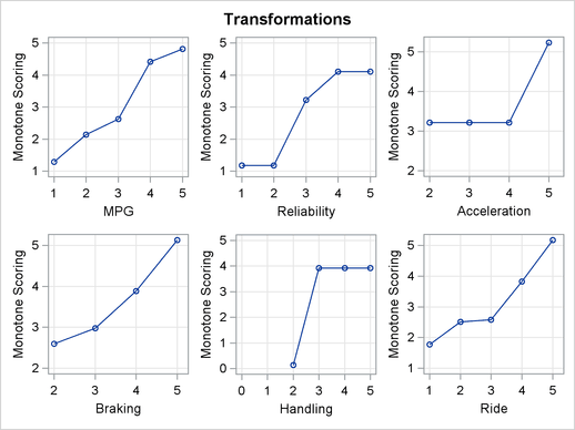
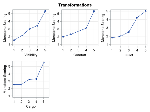
There are many patterns shown in the transformations in Figure 73.3. The transformation of Braking, for example, is not very different from the original scoring. The optimal scoring for other variables, such as Acceleration and Handling, is binary. Automobiles are differentiated by high versus everything else or low versus everything else.