The FACTOR Procedure
-
Overview

- Getting Started
-
Syntax
-
Details
Input Data Set Output Data Sets Confidence Intervals and the Salience of Factor Loadings Simplicity Functions for Rotations Missing Values Cautions Factor Scores Variable Weights and Variance Explained Heywood Cases and Other Anomalies about Communality Estimates Time Requirements Displayed Output ODS Table Names ODS Graphics
-
Examples
- References
Example 34.2 Principal Factor Analysis
This example uses the data presented in Example 34.1 and performs a principal factor analysis with squared multiple correlations for the prior communality estimates. Unlike Example 34.1, which analyzes the principal components (with default PRIORS=ONE), the current analysis is based on a common factor model. To use a common factor model, you specify PRIORS=SMC in the PROC FACTOR statement, as shown in the following:
ods graphics on;

proc factor data=SocioEconomics
   priors=smc msa residual
   rotate=promax reorder
   outstat=fact_all
   plots=(scree initloadings preloadings loadings);
run;
ods graphics off;
In the PROC FACTOR statement, you include several other options to help you analyze the results. To help determine whether the common factor model is appropriate, you request the Kaiser’s measure of sampling adequacy with the MSA option. You specify the RESIDUALS option to compute the residual correlations and partial correlations.
The ROTATE= and REORDER options are specified to enhance factor interpretability. The ROTATE=PROMAX option produces an orthogonal varimax prerotation (default) followed by an oblique Procrustes rotation, and the REORDER option reorders the variables according to their largest factor loadings. An OUTSTAT= data set is created by PROC FACTOR and displayed in Output 34.2.15.
PROC FACTOR can produce high-quality graphs that are very useful for interpreting the factor solutions. To request these graphs, ODS Graphics must be enabled. All ODS graphs in PROC FACTOR are requested with the PLOTS= option. In this example, you request a scree plot (SCREE) and loading plots for the factor matrix during the following three stages: initial unrotated solution (INITLOADINGS), prerotated (varimax) solution (PRELOADINGS), and promax-rotated solution (LOADINGS). The scree plot helps you determine the number of factors, and the loading plots help you visualize the patterns of factor loadings during various stages of analyses.
Principal Factor Analysis: Kaiser’s MSA and Factor Extraction Results
Output 34.2.1 displays the results of the partial correlations and Kaiser’s measure of sampling adequacy.
| Partial Correlations Controlling all other Variables | |||||
|---|---|---|---|---|---|
| Population | School | Employment | Services | HouseValue | |
| Population | 1.00000 | -0.54465 | 0.97083 | 0.09612 | 0.15871 |
| School | -0.54465 | 1.00000 | 0.54373 | 0.04996 | 0.64717 |
| Employment | 0.97083 | 0.54373 | 1.00000 | 0.06689 | -0.25572 |
| Services | 0.09612 | 0.04996 | 0.06689 | 1.00000 | 0.59415 |
| HouseValue | 0.15871 | 0.64717 | -0.25572 | 0.59415 | 1.00000 |
| Kaiser's Measure of Sampling Adequacy: Overall MSA = 0.57536759 | ||||
|---|---|---|---|---|
| Population | School | Employment | Services | HouseValue |
| 0.47207897 | 0.55158839 | 0.48851137 | 0.80664365 | 0.61281377 |
If the data are appropriate for the common factor model, the partial correlations (controlling all other variables) should be small compared to the original correlations. For example, the partial correlation between the variables School and HouseValue is  , slightly less than the original correlation of
  (see Output 34.1.3). The partial correlation between Population and School is
  , which is much larger in absolute value than the original correlation; this is an indication of trouble. Kaiser’s MSA is a summary, for each variable and for all variables together, of how much smaller the partial correlations are than the original correlations. Values of
  or
or  are considered good, while MSAs below
  are unacceptable. The variables Population, School, and Employment have very poor MSAs. Only the Services variable has a good MSA. The overall MSA of
  is sufficiently poor that additional variables should be included in the analysis to better define the common factors. A commonly used rule is that there should be at least three variables per factor. In the following analysis, you determine that there are two common factors in these data. Therefore, more variables are needed for a reliable analysis.
Output 34.2.2 displays the results of the principal factor extraction.
| Prior Communality Estimates: SMC | ||||
|---|---|---|---|---|
| Population | School | Employment | Services | HouseValue |
| 0.96859160 | 0.82228514 | 0.96918082 | 0.78572440 | 0.84701921 |
| Eigenvalues of the Reduced Correlation Matrix: Total = 4.39280116 Average = 0.87856023 | ||||
|---|---|---|---|---|
| Eigenvalue | Difference | Proportion | Cumulative | |
| 1 | 2.73430084 | 1.01823217 | 0.6225 | 0.6225 |
| 2 | 1.71606867 | 1.67650586 | 0.3907 | 1.0131 |
| 3 | 0.03956281 | 0.06408626 | 0.0090 | 1.0221 |
| 4 | -.02452345 | 0.04808427 | -0.0056 | 1.0165 |
| 5 | -.07260772 | -0.0165 | 1.0000 | |
The square multiple correlations are shown as prior communality estimates in Output 34.2.2. The PRIORS=SMC option basically replaces the diagonal of the original observed correlation matrix by these square multiple correlations. Because the square multiple correlations are usually less than one, the resulting correlation matrix for factoring is called the reduced correlation matrix. In the current example, the SMCs are all fairly large; hence, you expect the results of the principal factor analysis to be similar to those in the principal component analysis.
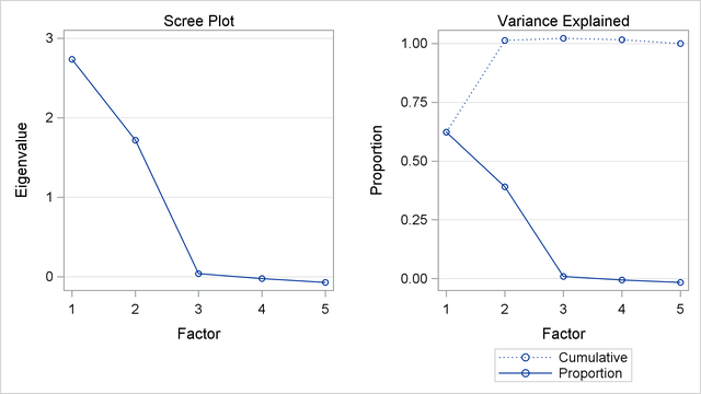
The first two largest positive eigenvalues of the reduced correlation matrix account for  of the common variance. This is possible because the reduced correlation matrix, in general, is not necessarily positive definite, and negative eigenvalues for the matrix are possible. A pattern like this suggests that you might not need more than two common factors. The scree and variance explained plots of Output 34.2.3 clearly support the conclusion that two common factors are present. Showing in the left panel of Output 34.2.3 is the scree plot of the eigenvalues of the reduced correlation matrix. A sharp bend occurs at the third eigenvalue, reinforcing the conclusion that two common factors are present. These cumulative proportions of common variance explained by factors are plotted in the right panel of Output 34.2.3, which shows that the curve essentially flattens out after the second factor.
Principal Factor Analysis: Initial Factor Solution
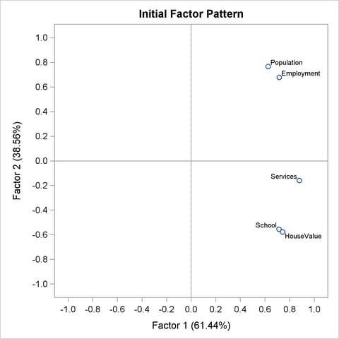
For the current analysis, PROC FACTOR retains two factors by certain default criteria. This decision agrees with the conclusion drawn by inspecting the scree plot. The principal factor pattern with the two factors is displayed in Output 34.2.4. This factor pattern is similar to the principal component pattern seen in Output 34.1.5 of Example 34.1. For example, the variable Services has the largest loading on the first factor, and the Population variable has the smallest. The variables Population and Employment have large positive loadings on the second factor, and the HouseValue and School variables have large negative loadings.
| Factor Pattern | ||
|---|---|---|
| Factor1 | Factor2 | |
| Services | 0.87899 | -0.15847 |
| HouseValue | 0.74215 | -0.57806 |
| Employment | 0.71447 | 0.67936 |
| School | 0.71370 | -0.55515 |
| Population | 0.62533 | 0.76621 |
| Variance Explained by Each Factor |
|
|---|---|
| Factor1 | Factor2 |
| 2.7343008 | 1.7160687 |
| Final Communality Estimates: Total = 4.450370 | ||||
|---|---|---|---|---|
| Population | School | Employment | Services | HouseValue |
| 0.97811334 | 0.81756387 | 0.97199928 | 0.79774304 | 0.88494998 |
Comparing the current factor loading matrix in Output 34.2.4 with that in Output 34.1.5 in Example 34.1, you notice that the variables are arranged differently in the two output tables. This is due to the use of the REORDER option in the current analysis. The advantage of using this option might not be very obvious in Output 34.2.4, but you can see its value when looking at the rotated solutions, as shown in Output 34.2.7 and Output 34.2.11.
The final communality estimates are all fairly close to the priors (shown in Output 34.2.2). Only the communality for the variable HouseValue increased appreciably, from  to
to  . Therefore, you are sure that all the common variance is accounted for.
Output 34.2.5 shows that the residual correlations (off-diagonal elements) are low, the largest being  . The partial correlations are not quite as impressive, since the uniqueness values are also rather small. These results indicate that the squared multiple correlations are good but not quite optimal communality estimates.
| Residual Correlations With Uniqueness on the Diagonal | |||||
|---|---|---|---|---|---|
| Population | School | Employment | Services | HouseValue | |
| Population | 0.02189 | -0.01118 | 0.00514 | 0.01063 | 0.00124 |
| School | -0.01118 | 0.18244 | 0.02151 | -0.02390 | 0.01248 |
| Employment | 0.00514 | 0.02151 | 0.02800 | -0.00565 | -0.01561 |
| Services | 0.01063 | -0.02390 | -0.00565 | 0.20226 | 0.03370 |
| HouseValue | 0.00124 | 0.01248 | -0.01561 | 0.03370 | 0.11505 |
| Root Mean Square Off-Diagonal Residuals: Overall = 0.01693282 | ||||
|---|---|---|---|---|
| Population | School | Employment | Services | HouseValue |
| 0.00815307 | 0.01813027 | 0.01382764 | 0.02151737 | 0.01960158 |
| Partial Correlations Controlling Factors | |||||
|---|---|---|---|---|---|
| Population | School | Employment | Services | HouseValue | |
| Population | 1.00000 | -0.17693 | 0.20752 | 0.15975 | 0.02471 |
| School | -0.17693 | 1.00000 | 0.30097 | -0.12443 | 0.08614 |
| Employment | 0.20752 | 0.30097 | 1.00000 | -0.07504 | -0.27509 |
| Services | 0.15975 | -0.12443 | -0.07504 | 1.00000 | 0.22093 |
| HouseValue | 0.02471 | 0.08614 | -0.27509 | 0.22093 | 1.00000 |
| Root Mean Square Off-Diagonal Partials: Overall = 0.18550132 | ||||
|---|---|---|---|---|
| Population | School | Employment | Services | HouseValue |
| 0.15850824 | 0.19025867 | 0.23181838 | 0.15447043 | 0.18201538 |
As displayed in Output 34.2.6, the unrotated factor pattern reveals two tight clusters of variables, with the variables HouseValue and School at the negative end of Factor2 axis and the variables Employment and Population at the positive end. The Services variable is in between but closer to the HouseValue and School variables. A good rotation would place the axes so that most variables would have zero loadings on most factors. As a result, the axes would appear as though they are put through the variable clusters.
Principal Factor Analysis: Varimax Prerotation
In Output 34.2.7, the results of the varimax prerotation are shown. To yield the varimax-rotated factor loading (pattern), the initial factor loading matrix is postmultiplied by an orthogonal transformation matrix. This orthogonal transformation matrix is shown in Output 34.2.7, followed by the varimax-rotated factor pattern. This rotation or transformation leads to small loadings of Population and Employment on the first factor and small loadings of HouseValue and School on the second factor. Services appears to have a larger loading on the first factor than it has on the second factor, although both loadings are substantial. Hence, Services appears to be factorially complex.
With the REORDER option in effect, you can see the variable clusters clearly in the factor pattern. The first factor is associated more with the first three variables (first three rows of variables): HouseValue, School, and Services. The second factor is associated more with the last two variables (last two rows of variables): Population and Employment.
For orthogonal factor solutions such as the current varimax-rotated solution, you can also interpret the values in the factor loading (pattern) matrix as correlations. For example, HouseValue and Factor 1 have a high correlation at  , while Population and Factor 1 have a low correlation at
  .
.
| Orthogonal Transformation Matrix | ||
|---|---|---|
| 1 | 2 | |
| 1 | 0.78895 | 0.61446 |
| 2 | -0.61446 | 0.78895 |
| Rotated Factor Pattern | ||
|---|---|---|
| Factor1 | Factor2 | |
| HouseValue | 0.94072 | -0.00004 |
| School | 0.90419 | 0.00055 |
| Services | 0.79085 | 0.41509 |
| Population | 0.02255 | 0.98874 |
| Employment | 0.14625 | 0.97499 |
| Variance Explained by Each Factor |
|
|---|---|
| Factor1 | Factor2 |
| 2.3498567 | 2.1005128 |
| Final Communality Estimates: Total = 4.450370 | ||||
|---|---|---|---|---|
| Population | School | Employment | Services | HouseValue |
| 0.97811334 | 0.81756387 | 0.97199928 | 0.79774304 | 0.88494998 |
The variance explained by the factors are more evenly distributed in the varimax-rotated solution, as compared with that of the unrotated solution. Indeed, this is a typical fact for any kinds of factor rotation. In the current example, before the varimax rotation the two factors explain  and
and  , respectively, of the common variance (see Output 34.2.4). After the varimax rotation the two rotated factors explain
  and
and  , respectively, of the common variance. However, the total variance accounted for by the factors remains unchanged after the varimax rotation. This invariance property is also observed for the communalities of the variables after the rotation, as evidenced by comparing the current communality estimates in Output 34.2.7 with those in Output 34.2.4.
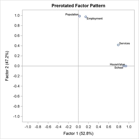
Output 34.2.8 shows the graphical plot of the varimax-rotated factor loadings. Clearly, HouseValue and School cluster together on the Factor 1 axis, while Population and Employment cluster together on the Factor 2 axis. Service is closer to the cluster of HouseValue and School.
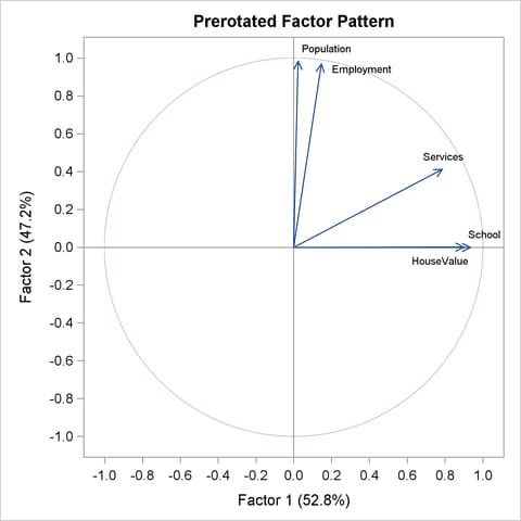
An alternative to the scatter plot of factor loadings is the so-called vector plot of loadings, which is shown in Output 34.2.9. The vector plot is requested with the suboption VECTOR in the PLOTS= option. That is:
plots=preloadings(vector)
This generates the vector plot of loadings in Output 34.2.9.
Principal Factor Analysis: Oblique Promax Rotation
For some researchers, the varimax-rotated factor solution in the preceding section might be good enough to provide them useful and interpretable results. For others who believe that common factors are seldom orthogonal, an obliquely rotated factor solution might be more desirable, or at least should be attempted.
PROC FACTOR provides a very large class of oblique factor rotations. The current example shows a particular one—namely, the promax rotation as requested by the ROTATE=PROMAX option.
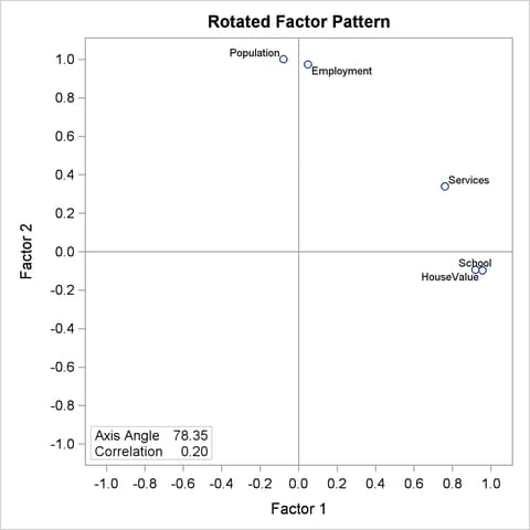
The results of the promax rotation are shown in Output 34.2.10 and Output 34.2.11. The corresponding plot of factor loadings is shown in Output 34.2.12.
| Target Matrix for Procrustean Transformation | ||
|---|---|---|
| Factor1 | Factor2 | |
| HouseValue | 1.00000 | -0.00000 |
| School | 1.00000 | 0.00000 |
| Services | 0.69421 | 0.10045 |
| Population | 0.00001 | 1.00000 |
| Employment | 0.00326 | 0.96793 |
| Procrustean Transformation Matrix | ||
|---|---|---|
| 1 | 2 | |
| 1 | 1.04116598 | -0.0986534 |
| 2 | -0.1057226 | 0.96303019 |
| Normalized Oblique Transformation Matrix |
||
|---|---|---|
| 1 | 2 | |
| 1 | 0.73803 | 0.54202 |
| 2 | -0.70555 | 0.86528 |
Output 34.2.10 shows the Procrustean target, to which the varimax factor pattern is rotated, followed by the display of the Procrustean transformation matrix. This is the matrix that transforms the varimax factor pattern so that the rotated pattern is as close as possible to the Procrustean target. However, because the variances of factors have to be fixed at 1 during the oblique transformation, a normalized version of the Procrustean transformation matrix is the one that is actually used in the transformation. This normalized transformation matrix is shown at the bottom of Output 34.2.10. Using this transformation matrix leads to the promax-rotated factor solution, as shown in Output 34.2.11.
| Inter-Factor Correlations | ||
|---|---|---|
| Factor1 | Factor2 | |
| Factor1 | 1.00000 | 0.20188 |
| Factor2 | 0.20188 | 1.00000 |
| Rotated Factor Pattern (Standardized Regression Coefficients) | ||
|---|---|---|
| Factor1 | Factor2 | |
| HouseValue | 0.95558485 | -0.0979201 |
| School | 0.91842142 | -0.0935214 |
| Services | 0.76053238 | 0.33931804 |
| Population | -0.0790832 | 1.00192402 |
| Employment | 0.04799 | 0.97509085 |
After the promax rotation, the factors are no longer uncorrelated. As shown in Output 34.2.11, the correlation of the two factors is now  . In the (initial) unrotated and the varimax solutions, the two factors are not correlated.
In addition to allowing the factors to be correlated, in an oblique factor solution you seek a pattern of factor loadings that is more "differentiated" (referred to as the "simple structures" in the literature). The more differentiated the loadings, the easier the interpretation of the factors.
For example, factor loadings of Services and Population on Factor 2 are  and
and  , respectively, in the (orthogonal) varimax-rotated factor pattern (see Output 34.2.7). With the (oblique) promax rotation (see Output 34.2.11), these two loadings become even more differentiated with values
  and
and  , respectively. Overall, however, the factor patterns before and after the promax rotation do not seem to differ too much. This fact is confirmed by comparing the graphical plots of factor loadings. The plots in Output 34.2.12 (promax-rotated factor loadings) and Output 34.2.8 (varimax-rotated factor loadings) show very similar patterns.
Unlike the orthogonal factor solutions where you can interpret the factor loadings as correlations between variables and factors, in oblique factor solutions such as the promax solution, you have to turn to the factor structure matrix for examining the correlations between variables and factors. Output 34.2.13 shows the factor structures of the promax-rotated solution.
| Factor Structure (Correlations) | ||
|---|---|---|
| Factor1 | Factor2 | |
| HouseValue | 0.93582 | 0.09500 |
| School | 0.89954 | 0.09189 |
| Services | 0.82903 | 0.49286 |
| Population | 0.12319 | 0.98596 |
| Employment | 0.24484 | 0.98478 |
| Variance Explained by Each Factor Ignoring Other Factors |
|
|---|---|
| Factor1 | Factor2 |
| 2.4473495 | 2.2022803 |
| Final Communality Estimates: Total = 4.450370 | ||||
|---|---|---|---|---|
| Population | School | Employment | Services | HouseValue |
| 0.97811334 | 0.81756387 | 0.97199928 | 0.79774304 | 0.88494998 |
Basically, the factor structure matrix shown in Output 34.2.13 reflects a similar pattern to the factor pattern matrix shown in Output 34.2.11. The critical difference is that you can have the correlation interpretation only by using the factor structure matrix. For example, in the factor structure matrix shown in Output 34.2.13, the correlation between Population and Factor 2 is  . The corresponding value shown in the factor pattern matrix in Output 34.2.11 is , which certainly cannot be interpreted as a correlation coefficient.
Common variance explained by the promax-rotated factors are 2.447 and 2.202, respectively, for the two factors. Unlike the orthogonal factor solutions (for example, the prerotated varimax solution), variance explained by these promax-rotated factors do not sum up to the total communality estimate 4.45. In oblique factor solutions, variance explained by oblique factors cannot be partitioned for the factors. Variance explained by a common factor is computed while ignoring the contributions from the other factors.
However, the communalities for the variables, as shown in the bottom of Output 34.2.13, do not change from rotation to rotation. They are still the same set of communalities in the initial, varimax-rotated, and promax-rotated solutions. This is a basic fact about factor rotations: they only redistribute the variance explained by the factors; the total variance explained by the factors for any variable (that is, the communality of the variable) remains unchanged.
In the literature of exploratory factor analysis, reference axes had been an important tool in factor rotation. Nowadays, rotations are seldom done through the uses of the reference axes. Despite that, results about reference axes do provide additional information for interpreting factor analysis results. For the current example of the promax rotation, PROC FACTOR shows the relevant results about the reference axes in Output 34.2.14.
| Reference Axis Correlations | ||
|---|---|---|
| Factor1 | Factor2 | |
| Factor1 | 1.00000 | -0.20188 |
| Factor2 | -0.20188 | 1.00000 |
| Reference Structure (Semipartial Correlations) | ||
|---|---|---|
| Factor1 | Factor2 | |
| HouseValue | 0.93591 | -0.09590 |
| School | 0.89951 | -0.09160 |
| Services | 0.74487 | 0.33233 |
| Population | -0.07745 | 0.98129 |
| Employment | 0.04700 | 0.95501 |
| Variance Explained by Each Factor Eliminating Other Factors |
|
|---|---|
| Factor1 | Factor2 |
| 2.2480892 | 2.0030200 |
To explain the results in the reference-axis system, some geometric interpretations of the factor axes are needed. Consider a single factor in a system of  common factors in an oblique factor solution. Taking away the factor under consideration, the remaining
  factors span a hyperplane in the factor space of dimensions. The vector that is orthogonal to this hyperplane is the reference axis (reference vector) of the factor under consideration. Using the same definition for the remaining factors, you have reference vectors for factors.
A factor in an oblique factor solution can be considered as the sum of two independent components: its associated reference vector and a component that is overlapped with all other factors. In other words, the reference vector of a factor is a unique part of the factor that is not predictable from all other factors. Thus, the loadings on a reference vector are the unique effects of the corresponding factor, partialling out the effects from all other factors. The variances explained by a reference vector are the unique variances explained by the corresponding factor, partialling out the variances explained by all other factors.
Output 34.2.14 shows the reference axis correlations. The correlation between the reference vectors is  . Next, Output 34.2.14 shows the loadings on the reference vectors in the table entitled "Reference Structure (Semipartial Correlations)." As explained previously, loadings on a reference vector are also the unique effects of the corresponding factor, partialling out the effects from the all other factors. For example, the unique effect of Factor 1 on HouseValue is
  . Another important property of the reference vector system is that loadings on a reference vector are also correlations between the variables and the corresponding factor, partialling out the correlations between the variables and other factors. This means that the loading 0.936 in the reference structure table is the unique correlation between HouseValue and Factor 1, partialling out the correlation between HouseValue with Factor 2. Hence, as suggested by the title of table, all loadings reported in the "Reference Structure (Semipartial Correlations)" can be interpreted as semipartial correlations between variables and factors.
The last table shown in Output 34.2.14 are the variances explained by the reference vectors. As explained previously, these are also unique variances explained by the factors, partialling out the variances explained by all other factors (or eliminating all other factors, as suggested by the title of the table). In the current example, Factor 1 explains  of the variable variances, partialling out all variable variances explained by Factor 2.
Notice that factor pattern (shown in Output 34.2.11), factor structures (correlations, shown in Output 34.2.13), and reference structures (semipartial correlations, shown in Output 34.2.14) give you different information about the oblique factor solutions such as the promax-rotated solution. However, for orthogonal factor solutions such as the varimax-rotated solution, factor structures and reference structures are all the same as the factor pattern.
Principal Factor Analysis: Factor Rotations with Factor Pattern Input
The promax rotation is one of the many rotations that PROC FACTOR provides. You can specify many different rotation algorithms by using the ROTATE= options. In this section, you explore different rotated factor solutions from the initial principal factor solution. Specifically, you want to examine the factor patterns yielded by the quartimax transformation (an orthogonal transformation) and the Harris-Kaiser (an oblique transformation), respectively.
Rather than analyzing the entire problem again with new rotations, you can simply use the OUTSTAT= data set from the preceding factor analysis results.
First, the OUTSTAT= data set is printed using the following statements:
proc print data=fact_all;
run;
The output data set is displayed in Output 34.2.15.
| Factor Output Data Set |
| Obs | _TYPE_ | _NAME_ | Population | School | Employment | Services | HouseValue |
|---|---|---|---|---|---|---|---|
| 1 | MEAN | 6241.67 | 11.4417 | 2333.33 | 120.833 | 17000.00 | |
| 2 | STD | 3439.99 | 1.7865 | 1241.21 | 114.928 | 6367.53 | |
| 3 | N | 12.00 | 12.0000 | 12.00 | 12.000 | 12.00 | |
| 4 | CORR | Population | 1.00 | 0.0098 | 0.97 | 0.439 | 0.02 |
| 5 | CORR | School | 0.01 | 1.0000 | 0.15 | 0.691 | 0.86 |
| 6 | CORR | Employment | 0.97 | 0.1543 | 1.00 | 0.515 | 0.12 |
| 7 | CORR | Services | 0.44 | 0.6914 | 0.51 | 1.000 | 0.78 |
| 8 | CORR | HouseValue | 0.02 | 0.8631 | 0.12 | 0.778 | 1.00 |
| 9 | COMMUNAL | 0.98 | 0.8176 | 0.97 | 0.798 | 0.88 | |
| 10 | PRIORS | 0.97 | 0.8223 | 0.97 | 0.786 | 0.85 | |
| 11 | EIGENVAL | 2.73 | 1.7161 | 0.04 | -0.025 | -0.07 | |
| 12 | UNROTATE | Factor1 | 0.63 | 0.7137 | 0.71 | 0.879 | 0.74 |
| 13 | UNROTATE | Factor2 | 0.77 | -0.5552 | 0.68 | -0.158 | -0.58 |
| 14 | RESIDUAL | Population | 0.02 | -0.0112 | 0.01 | 0.011 | 0.00 |
| 15 | RESIDUAL | School | -0.01 | 0.1824 | 0.02 | -0.024 | 0.01 |
| 16 | RESIDUAL | Employment | 0.01 | 0.0215 | 0.03 | -0.006 | -0.02 |
| 17 | RESIDUAL | Services | 0.01 | -0.0239 | -0.01 | 0.202 | 0.03 |
| 18 | RESIDUAL | HouseValue | 0.00 | 0.0125 | -0.02 | 0.034 | 0.12 |
| 19 | PRETRANS | Factor1 | 0.79 | -0.6145 | . | . | . |
| 20 | PRETRANS | Factor2 | 0.61 | 0.7889 | . | . | . |
| 21 | PREROTAT | Factor1 | 0.02 | 0.9042 | 0.15 | 0.791 | 0.94 |
| 22 | PREROTAT | Factor2 | 0.99 | 0.0006 | 0.97 | 0.415 | -0.00 |
| 23 | TRANSFOR | Factor1 | 0.74 | -0.7055 | . | . | . |
| 24 | TRANSFOR | Factor2 | 0.54 | 0.8653 | . | . | . |
| 25 | FCORR | Factor1 | 1.00 | 0.2019 | . | . | . |
| 26 | FCORR | Factor2 | 0.20 | 1.0000 | . | . | . |
| 27 | PATTERN | Factor1 | -0.08 | 0.9184 | 0.05 | 0.761 | 0.96 |
| 28 | PATTERN | Factor2 | 1.00 | -0.0935 | 0.98 | 0.339 | -0.10 |
| 29 | RCORR | Factor1 | 1.00 | -0.2019 | . | . | . |
| 30 | RCORR | Factor2 | -0.20 | 1.0000 | . | . | . |
| 31 | REFERENC | Factor1 | -0.08 | 0.8995 | 0.05 | 0.745 | 0.94 |
| 32 | REFERENC | Factor2 | 0.98 | -0.0916 | 0.96 | 0.332 | -0.10 |
| 33 | STRUCTUR | Factor1 | 0.12 | 0.8995 | 0.24 | 0.829 | 0.94 |
| 34 | STRUCTUR | Factor2 | 0.99 | 0.0919 | 0.98 | 0.493 | 0.09 |
Various results from the previous factor analysis are saved in this data set, including the initial unrotated solution (its factor pattern is saved in observations with _TYPE_=UNROTATE), the prerotated varimax solution (its factor pattern is saved in observations with _TYPE_=PREROTAT), and the oblique promax solution (its factor pattern is saved in observations with _TYPE_=PATTERN).
When PROC FACTOR reads in an input data set with TYPE=FACTOR, the observations with _TYPE_=PATTERN are treated as the initial factor pattern to be rotated by PROC FACTOR. Hence, it is important that you provide the correct initial factor pattern for PROC FACTOR to read in.
In the current example, you need to provide the unrotated solution from the preceding analysis as the input factor pattern. The following statements create a TYPE=FACTOR data set fact2 from the preceding OUTSTAT= data set fact_all:
data fact2(type=factor);
   set fact_all;
   if _TYPE_ in('PATTERN' 'FCORR') then delete;
   if _TYPE_='UNROTATE' then _TYPE_='PATTERN';
In these statements, you delete observations with _TYPE_=PATTERN or _TYPE_=FCORR, which are for the promax-rotated factor solution, and change observations with _TYPE_=UNROTATE to _TYPE_=PATTERN in the new data set fact2. In this way, the initial orthogonal factor pattern matrix is saved in the observations with _TYPE_=PATTERN.
You use this new data set and rotate the initial solution to another oblique solution with the ROTATE=QUARTIMAX option, as shown in the following statements:
proc factor data=fact2 rotate=quartimax reorder;
run;
As shown in Output 34.2.16, the input data set is of the FACTOR type for the new rotation.
| Quartimax Rotation From a TYPE=FACTOR Data Set |
| Input Data Type | FACTOR |
|---|---|
| N Set/Assumed in Data Set | 12 |
| N for Significance Tests | 12 |
The quartimax-rotated factor pattern is displayed in Output 34.2.17.
| Orthogonal Transformation Matrix | ||
|---|---|---|
| 1 | 2 | |
| 1 | 0.80138 | 0.59815 |
| 2 | -0.59815 | 0.80138 |
| Rotated Factor Pattern | ||
|---|---|---|
| Factor1 | Factor2 | |
| HouseValue | 0.94052 | -0.01933 |
| School | 0.90401 | -0.01799 |
| Services | 0.79920 | 0.39878 |
| Population | 0.04282 | 0.98807 |
| Employment | 0.16621 | 0.97179 |
| Variance Explained by Each Factor |
|
|---|---|
| Factor1 | Factor2 |
| 2.3699941 | 2.0803754 |
The quartimax rotation produces an orthogonal transformation matrix shown at the top of Output 34.2.17. After the transformation, the factor pattern is shown next. Compared with the varimax-rotated factor pattern (see Output 34.2.7), the quartimax-rotated factor pattern shows some differences. The loadings of HouseValue and School on Factor 1 drop only slightly in the quartimax factor pattern, while the loadings of Services, Population, and Employment on Factor 1 gain relatively larger amounts. The total variance explained by Factor 1 in the varimax-rotated solution (see Output 34.2.7) is  , while it is
  after the quartimax-rotation. In other words, more variable variances are explained by the first factor in the quartimax factor pattern than in the varimax factor pattern. Although not very strongly demonstrated in the current example, this illustrates a well-known property about the quartimax rotation: it tends to produce a general factor for all variables.
Another oblique rotation is now explored. The Harris-Kaiser transformation weighted by the Cureton-Mulaik technique is applied to the initial factor pattern. To achieve this, you use the ROTATE=HK and NORM=WEIGHT options in the following PROC FACTOR statement:
ods graphics on;
proc factor data=fact2 rotate=hk norm=weight reorder
     plots=loadings;
run;

ods graphics off;
Output 34.2.18 shows the variable weights in the rotation.
| Variable Weights for Rotation | ||||
|---|---|---|---|---|
| Population | School | Employment | Services | HouseValue |
| 0.95982747 | 0.93945424 | 0.99746396 | 0.12194766 | 0.94007263 |
While all other variables have weights at least as large as  , the weight for Services is only
  . This means that due to its small weight, Services is not as important as the other variables for determining the rotation (transformation). This makes sense when you look at the initial unrotated factor pattern plot in Output 34.2.6. In the plot, there are two main clusters of variables, and Services does not seem to fall into either of the clusters. In order to yield a Harris-Kaiser rotation (transformation) that would gear towards to two clusters, the Cureton-Mulaik weighting essentially downweights the contribution from Services in the factor rotation.
The results of the Harris-Kaiser factor solution are displayed in Output 34.2.19, with a graphical plot of rotated loadings displayed in Output 34.2.20.
| Inter-Factor Correlations | ||
|---|---|---|
| Factor1 | Factor2 | |
| Factor1 | 1.00000 | 0.08358 |
| Factor2 | 0.08358 | 1.00000 |
| Rotated Factor Pattern (Standardized Regression Coefficients) | ||
|---|---|---|
| Factor1 | Factor2 | |
| HouseValue | 0.94048 | 0.00279 |
| School | 0.90391 | 0.00327 |
| Services | 0.75459 | 0.41892 |
| Population | -0.06335 | 0.99227 |
| Employment | 0.06152 | 0.97885 |
Because the Harris-Kaiser produces an oblique factor solution, you compare the current results with that of the promax (see Output 34.2.11), which also produces an oblique factor solution. The correlation between the factors in the Harris-Kaiser solution is  ; this value is much smaller than the same correlation in the promax solution, which is
  . However, the Harris-Kaiser rotated factor pattern shown in Output 34.2.19 is more or less the same as that of the promax-rotated factor pattern shown in Output 34.2.11. Which solution would you consider to be more reasonable or interpretable?
From the statistical point of view, the Harris-Kaiser and promax factor solutions are equivalent. They explain the observed variable relationships equally well. From the simplicity point of view, however, you might prefer to interpret the Harris-Kaiser solution because the factor correlation is smaller. In other words, the factors in the Harris-Kaiser solution do not overlap that much conceptually; hence they should be more distinctive to interpret. However, in practice simplicity in factor correlations might not the only principle to consider. Researchers might actually expect to have some factors to be highly correlated based on theoretical or substantive grounds.
Although the Harris-Kaiser and the promax factor patterns are very similar, the graphical plots of the loadings from the two solutions paint slightly different pictures. The plot of the promax-rotated loadings is shown in Output 34.2.12, while the plot of the loadings for the current Harris-Kaiser solution is shown in Output 34.2.20.
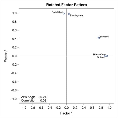
The two factor axes in the Harris-Kaiser rotated pattern (Output 34.2.20) clearly cut through the centers of the two variable clusters, while the Factor 1 axis in the promax solution lies above a variable cluster (Output 34.2.12). The reason for this subtle difference is that in the Harris-Kaiser rotation, the Services is a "loner" that has been downweighted by the Cureton-Mulaik technique (see its relatively small weight in Output 34.2.18). As a result, the rotated axes are basically determined by the two variable clusters in the Harris-Kaiser rotation.
As far as the current discussion goes, it is not recommending one rotation method over another. Rather, it simply illustrates how you could control certain types of characteristics of factor rotation through the many options supported by PROC FACTOR. Should you prefer an orthogonal rotation to an oblique rotation? Should you choose the oblique factor solution with the smallest factor correlations? Should you use a weighting scheme that would enable you to find independent variable clusters? While PROC FACTOR enables you to explore all these alternatives, you must consult advanced textbooks and published articles to get satisfactory and complete answers to these questions.