The CORRESP Procedure

Example 31.1 Simple and Multiple Correspondence Analysis of Automobiles and Their Owners
In this example, PROC CORRESP creates a contingency table from categorical data and performs a simple correspondence analysis. The data are from a sample of individuals who were asked to provide information about themselves and their automobiles. The questions included origin of the automobile (American, Japanese, European) and family status (single, married, single and living with children, married living with children).
The first steps read the input data and assign formats. PROC CORRESP is used to perform the simple correspondence analysis. The ALL option displays all tables, including the contingency table, chi-square information, profiles, and all results of the correspondence analysis. The OUTC= option creates an output coordinate data set. The TABLES statement specifies the row and column categorical variables. The results are displayed with ODS Graphics.
The following statements produce Output 31.1.1:
title1 'Automobile Owners and Auto Attributes';
title2 'Simple Correspondence Analysis';

proc format;
   value Origin  1 = 'American' 2 = 'Japanese' 3 = 'European';
   value Size    1 = 'Small'    2 = 'Medium'   3 = 'Large';
   value Type    1 = 'Family'   2 = 'Sporty'   3 = 'Work';
   value Home    1 = 'Own'      2 = 'Rent';
   value Sex     1 = 'Male'     2 = 'Female';
   value Income  1 = '1 Income' 2 = '2 Incomes';
   value Marital 1 = 'Single with Kids' 2 = 'Married with Kids'
                 3 = 'Single'           4 = 'Married';
run;

data Cars;
   missing a;
   input (Origin Size Type Home Income Marital Kids Sex) (1.) @@;
   * Check for End of Line;
   if n(of Origin -- Sex) eq 0 then do; input; return; end;
   marital = 2 * (kids le 0) + marital;
   format Origin Origin. Size Size. Type Type. Home Home.
          Sex Sex. Income Income. Marital Marital.;
   output;
   datalines;
131112212121110121112201131211011211221122112121131122123211222212212201
121122023121221232211101122122022121110122112102131112211121110112311101
211112113211223121122202221122111311123131211102321122223221220221221101

   ... more lines ...

212122011211122131221101121211022212220212121101
;
ods graphics on;

* Perform Simple Correspondence Analysis;
proc corresp all data=Cars outc=Coor;
   tables Marital, Origin;
run;
Correspondence analysis locates all the categories in a Euclidean space. The first two dimensions of this space are plotted to examine the associations among the categories. Since the smallest dimension of this table is three, there is no loss of information when only two dimensions are plotted. The plot should be thought of as two different overlaid plots, one for each categorical variable. Distances between points within a variable have meaning, but distances between points from different variables do not.
| Automobile Owners and Auto Attributes |
| Simple Correspondence Analysis |
| Contingency Table | ||||
|---|---|---|---|---|
| American | European | Japanese | Sum | |
| Married | 37 | 14 | 51 | 102 |
| Married with Kids | 52 | 15 | 44 | 111 |
| Single | 33 | 15 | 63 | 111 |
| Single with Kids | 6 | 1 | 8 | 15 |
| Sum | 128 | 45 | 166 | 339 |
| Chi-Square Statistic Expected Values | |||
|---|---|---|---|
| American | European | Japanese | |
| Married | 38.5133 | 13.5398 | 49.9469 |
| Married with Kids | 41.9115 | 14.7345 | 54.3540 |
| Single | 41.9115 | 14.7345 | 54.3540 |
| Single with Kids | 5.6637 | 1.9912 | 7.3451 |
| Observed Minus Expected Values | |||
|---|---|---|---|
| American | European | Japanese | |
| Married | -1.5133 | 0.4602 | 1.0531 |
| Married with Kids | 10.0885 | 0.2655 | -10.3540 |
| Single | -8.9115 | 0.2655 | 8.6460 |
| Single with Kids | 0.3363 | -0.9912 | 0.6549 |
| Contributions to the Total Chi-Square Statistic | ||||
|---|---|---|---|---|
| American | European | Japanese | Sum | |
| Married | 0.05946 | 0.01564 | 0.02220 | 0.09730 |
| Married with Kids | 2.42840 | 0.00478 | 1.97235 | 4.40553 |
| Single | 1.89482 | 0.00478 | 1.37531 | 3.27492 |
| Single with Kids | 0.01997 | 0.49337 | 0.05839 | 0.57173 |
| Sum | 4.40265 | 0.51858 | 3.42825 | 8.34947 |
| Row Profiles | |||
|---|---|---|---|
| American | European | Japanese | |
| Married | 0.362745 | 0.137255 | 0.500000 |
| Married with Kids | 0.468468 | 0.135135 | 0.396396 |
| Single | 0.297297 | 0.135135 | 0.567568 |
| Single with Kids | 0.400000 | 0.066667 | 0.533333 |
| Column Profiles | |||
|---|---|---|---|
| American | European | Japanese | |
| Married | 0.289063 | 0.311111 | 0.307229 |
| Married with Kids | 0.406250 | 0.333333 | 0.265060 |
| Single | 0.257813 | 0.333333 | 0.379518 |
| Single with Kids | 0.046875 | 0.022222 | 0.048193 |
| Automobile Owners and Auto Attributes |
| Simple Correspondence Analysis |
| Inertia and Chi-Square Decomposition | |||||
|---|---|---|---|---|---|
| Singular Value |
Principal Inertia |
Chi- Square |
Percent |
Cumulative Percent |
19 38 57 76 95 ----+----+----+----+----+--- |
| 0.15122 | 0.02287 | 7.75160 | 92.84 | 92.84 | ************************ |
| 0.04200 | 0.00176 | 0.59787 | 7.16 | 100.00 | ** |
| Total | 0.02463 | 8.34947 | 100.00 | ||
| Degrees of Freedom = 6 | |||||
| Row Coordinates | ||
|---|---|---|
| Dim1 | Dim2 | |
| Married | -0.0278 | 0.0134 |
| Married with Kids | 0.1991 | 0.0064 |
| Single | -0.1716 | 0.0076 |
| Single with Kids | -0.0144 | -0.1947 |
| Summary Statistics for the Row Points | |||
|---|---|---|---|
| Quality | Mass | Inertia | |
| Married | 1.0000 | 0.3009 | 0.0117 |
| Married with Kids | 1.0000 | 0.3274 | 0.5276 |
| Single | 1.0000 | 0.3274 | 0.3922 |
| Single with Kids | 1.0000 | 0.0442 | 0.0685 |
| Partial Contributions to Inertia for the Row Points |
||
|---|---|---|
| Dim1 | Dim2 | |
| Married | 0.0102 | 0.0306 |
| Married with Kids | 0.5678 | 0.0076 |
| Single | 0.4217 | 0.0108 |
| Single with Kids | 0.0004 | 0.9511 |
| Indices of the Coordinates That Contribute Most to Inertia for the Row Points | |||
|---|---|---|---|
| Dim1 | Dim2 | Best | |
| Married | 0 | 0 | 2 |
| Married with Kids | 1 | 0 | 1 |
| Single | 1 | 0 | 1 |
| Single with Kids | 0 | 2 | 2 |
| Squared Cosines for the Row Points | ||
|---|---|---|
| Dim1 | Dim2 | |
| Married | 0.8121 | 0.1879 |
| Married with Kids | 0.9990 | 0.0010 |
| Single | 0.9980 | 0.0020 |
| Single with Kids | 0.0054 | 0.9946 |
| Column Coordinates | ||
|---|---|---|
| Dim1 | Dim2 | |
| American | 0.1847 | -0.0166 |
| European | 0.0013 | 0.1073 |
| Japanese | -0.1428 | -0.0163 |
| Summary Statistics for the Column Points |
|||
|---|---|---|---|
| Quality | Mass | Inertia | |
| American | 1.0000 | 0.3776 | 0.5273 |
| European | 1.0000 | 0.1327 | 0.0621 |
| Japanese | 1.0000 | 0.4897 | 0.4106 |
| Partial Contributions to Inertia for the Column Points |
||
|---|---|---|
| Dim1 | Dim2 | |
| American | 0.5634 | 0.0590 |
| European | 0.0000 | 0.8672 |
| Japanese | 0.4366 | 0.0737 |
| Indices of the Coordinates That Contribute Most to Inertia for the Column Points |
|||
|---|---|---|---|
| Dim1 | Dim2 | Best | |
| American | 1 | 0 | 1 |
| European | 0 | 2 | 2 |
| Japanese | 1 | 0 | 1 |
| Squared Cosines for the Column Points |
||
|---|---|---|
| Dim1 | Dim2 | |
| American | 0.9920 | 0.0080 |
| European | 0.0001 | 0.9999 |
| Japanese | 0.9871 | 0.0129 |
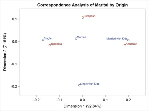
To interpret the plot, start by interpreting the row points separately from the column points. The European point is near and to the left of the centroid, so it makes a relatively small contribution to the chi-square statistic (because it is near the centroid), it contributes almost nothing to the inertia of dimension one (since its coordinate on dimension one has a small absolute value relative to the other column points), and it makes a relatively large contribution to the inertia of dimension two (since its coordinate on dimension two has a large absolute value relative to the other column points). Its squared cosines for dimension one and two, approximately 0 and 1, respectively, indicate that its position is almost completely determined by its location on dimension two. Its quality of display is 1.0, indicating perfect quality, since the table is two-dimensional after the centering. The American and Japanese points are far from the centroid, and they lie along dimension one. They make relatively large contributions to the chi-square statistic and the inertia of dimension one. The horizontal dimension seems to be largely determined by Japanese versus American automobile ownership.
In the row points, the Married point is near the centroid, and the Single with Kids point has a small coordinate on dimension one that is near zero. The horizontal dimension seems to be largely determined by the Single versus the Married with Kids points. The two interpretations of dimension one show the association with being Married with Kids and owning an American auto, and being single and owning a Japanese auto. The fact that the Married with Kids point is close to the American point and the fact that the Japanese point is near the Single point should be ignored. Distances between row and column points are not defined. The plot shows that more people who are married with kids than you would expect if the rows and columns were independent drive an American auto, and more people who are single than you would expect if the rows and columns were independent drive a Japanese auto.
In the second part of this example, PROC CORRESP creates a Burt table from categorical data and performs a multiple correspondence analysis. The variables used in this example are Origin, Size, Type, Income, Home, Marital, and Sex. MCA specifies multiple correspondence analysis, OBSERVED displays the Burt table, and the OUTC= option creates an output coordinate data set. The TABLES statement with only a single variable list and no comma creates the Burt table.
The following statements produce Output 31.1.2:
title2 'Multiple Correspondence Analysis';

* Perform Multiple Correspondence Analysis;
proc corresp mca observed data=Cars outc=Coor;
   tables Origin Size Type Income Home Marital Sex;
run;
| Automobile Owners and Auto Attributes |
| Multiple Correspondence Analysis |
| Burt Table | |||||||||||||||||||
|---|---|---|---|---|---|---|---|---|---|---|---|---|---|---|---|---|---|---|---|
| American | European | Japanese | Large | Medium | Small | Family | Sporty | Work | 1 Income | 2 Incomes | Own | Rent | Married | Married with Kids |
Single | Single with Kids |
Female | Male | |
| American | 125 | 0 | 0 | 36 | 60 | 29 | 81 | 24 | 20 | 58 | 67 | 93 | 32 | 37 | 50 | 32 | 6 | 58 | 67 |
| European | 0 | 44 | 0 | 4 | 20 | 20 | 17 | 23 | 4 | 18 | 26 | 38 | 6 | 13 | 15 | 15 | 1 | 21 | 23 |
| Japanese | 0 | 0 | 165 | 2 | 61 | 102 | 76 | 59 | 30 | 74 | 91 | 111 | 54 | 51 | 44 | 62 | 8 | 70 | 95 |
| Large | 36 | 4 | 2 | 42 | 0 | 0 | 30 | 1 | 11 | 20 | 22 | 35 | 7 | 9 | 21 | 11 | 1 | 17 | 25 |
| Medium | 60 | 20 | 61 | 0 | 141 | 0 | 89 | 39 | 13 | 57 | 84 | 106 | 35 | 42 | 51 | 40 | 8 | 70 | 71 |
| Small | 29 | 20 | 102 | 0 | 0 | 151 | 55 | 66 | 30 | 73 | 78 | 101 | 50 | 50 | 37 | 58 | 6 | 62 | 89 |
| Family | 81 | 17 | 76 | 30 | 89 | 55 | 174 | 0 | 0 | 69 | 105 | 130 | 44 | 50 | 79 | 35 | 10 | 83 | 91 |
| Sporty | 24 | 23 | 59 | 1 | 39 | 66 | 0 | 106 | 0 | 55 | 51 | 71 | 35 | 35 | 12 | 57 | 2 | 44 | 62 |
| Work | 20 | 4 | 30 | 11 | 13 | 30 | 0 | 0 | 54 | 26 | 28 | 41 | 13 | 16 | 18 | 17 | 3 | 22 | 32 |
| 1 Income | 58 | 18 | 74 | 20 | 57 | 73 | 69 | 55 | 26 | 150 | 0 | 80 | 70 | 10 | 27 | 99 | 14 | 47 | 103 |
| 2 Incomes | 67 | 26 | 91 | 22 | 84 | 78 | 105 | 51 | 28 | 0 | 184 | 162 | 22 | 91 | 82 | 10 | 1 | 102 | 82 |
| Own | 93 | 38 | 111 | 35 | 106 | 101 | 130 | 71 | 41 | 80 | 162 | 242 | 0 | 76 | 106 | 52 | 8 | 114 | 128 |
| Rent | 32 | 6 | 54 | 7 | 35 | 50 | 44 | 35 | 13 | 70 | 22 | 0 | 92 | 25 | 3 | 57 | 7 | 35 | 57 |
| Married | 37 | 13 | 51 | 9 | 42 | 50 | 50 | 35 | 16 | 10 | 91 | 76 | 25 | 101 | 0 | 0 | 0 | 53 | 48 |
| Married with Kids | 50 | 15 | 44 | 21 | 51 | 37 | 79 | 12 | 18 | 27 | 82 | 106 | 3 | 0 | 109 | 0 | 0 | 48 | 61 |
| Single | 32 | 15 | 62 | 11 | 40 | 58 | 35 | 57 | 17 | 99 | 10 | 52 | 57 | 0 | 0 | 109 | 0 | 35 | 74 |
| Single with Kids | 6 | 1 | 8 | 1 | 8 | 6 | 10 | 2 | 3 | 14 | 1 | 8 | 7 | 0 | 0 | 0 | 15 | 13 | 2 |
| Female | 58 | 21 | 70 | 17 | 70 | 62 | 83 | 44 | 22 | 47 | 102 | 114 | 35 | 53 | 48 | 35 | 13 | 149 | 0 |
| Male | 67 | 23 | 95 | 25 | 71 | 89 | 91 | 62 | 32 | 103 | 82 | 128 | 57 | 48 | 61 | 74 | 2 | 0 | 185 |
| Automobile Owners and Auto Attributes |
| Multiple Correspondence Analysis |
| Inertia and Chi-Square Decomposition | |||||
|---|---|---|---|---|---|
| Singular Value |
Principal Inertia |
Chi- Square |
Percent |
Cumulative Percent |
4 8 12 16 20 ----+----+----+----+----+--- |
| 0.56934 | 0.32415 | 970.77 | 18.91 | 18.91 | ************************ |
| 0.48352 | 0.23380 | 700.17 | 13.64 | 32.55 | ***************** |
| 0.42716 | 0.18247 | 546.45 | 10.64 | 43.19 | ************* |
| 0.41215 | 0.16987 | 508.73 | 9.91 | 53.10 | ************ |
| 0.38773 | 0.15033 | 450.22 | 8.77 | 61.87 | *********** |
| 0.38520 | 0.14838 | 444.35 | 8.66 | 70.52 | *********** |
| 0.34066 | 0.11605 | 347.55 | 6.77 | 77.29 | ******** |
| 0.32983 | 0.10879 | 325.79 | 6.35 | 83.64 | ******** |
| 0.31517 | 0.09933 | 297.47 | 5.79 | 89.43 | ******* |
| 0.28069 | 0.07879 | 235.95 | 4.60 | 94.03 | ****** |
| 0.26115 | 0.06820 | 204.24 | 3.98 | 98.01 | ***** |
| 0.18477 | 0.03414 | 102.24 | 1.99 | 100.00 | ** |
| Total | 1.71429 | 5133.92 | 100.00 | ||
| Degrees of Freedom = 324 | |||||
| Column Coordinates | ||
|---|---|---|
| Dim1 | Dim2 | |
| American | -0.4035 | 0.8129 |
| European | -0.0568 | -0.5552 |
| Japanese | 0.3208 | -0.4678 |
| Large | -0.6949 | 1.5666 |
| Medium | -0.2562 | 0.0965 |
| Small | 0.4326 | -0.5258 |
| Family | -0.4201 | 0.3602 |
| Sporty | 0.6604 | -0.6696 |
| Work | 0.0575 | 0.1539 |
| 1 Income | 0.8251 | 0.5472 |
| 2 Incomes | -0.6727 | -0.4461 |
| Own | -0.3887 | -0.0943 |
| Rent | 1.0225 | 0.2480 |
| Married | -0.4169 | -0.7954 |
| Married with Kids | -0.8200 | 0.3237 |
| Single | 1.1461 | 0.2930 |
| Single with Kids | 0.4373 | 0.8736 |
| Female | -0.3365 | -0.2057 |
| Male | 0.2710 | 0.1656 |
| Summary Statistics for the Column Points | |||
|---|---|---|---|
| Quality | Mass | Inertia | |
| American | 0.4925 | 0.0535 | 0.0521 |
| European | 0.0473 | 0.0188 | 0.0724 |
| Japanese | 0.3141 | 0.0706 | 0.0422 |
| Large | 0.4224 | 0.0180 | 0.0729 |
| Medium | 0.0548 | 0.0603 | 0.0482 |
| Small | 0.3825 | 0.0646 | 0.0457 |
| Family | 0.3330 | 0.0744 | 0.0399 |
| Sporty | 0.4112 | 0.0453 | 0.0569 |
| Work | 0.0052 | 0.0231 | 0.0699 |
| 1 Income | 0.7991 | 0.0642 | 0.0459 |
| 2 Incomes | 0.7991 | 0.0787 | 0.0374 |
| Own | 0.4208 | 0.1035 | 0.0230 |
| Rent | 0.4208 | 0.0393 | 0.0604 |
| Married | 0.3496 | 0.0432 | 0.0581 |
| Married with Kids | 0.3765 | 0.0466 | 0.0561 |
| Single | 0.6780 | 0.0466 | 0.0561 |
| Single with Kids | 0.0449 | 0.0064 | 0.0796 |
| Female | 0.1253 | 0.0637 | 0.0462 |
| Male | 0.1253 | 0.0791 | 0.0372 |
| Partial Contributions to Inertia for the Column Points |
||
|---|---|---|
| Dim1 | Dim2 | |
| American | 0.0268 | 0.1511 |
| European | 0.0002 | 0.0248 |
| Japanese | 0.0224 | 0.0660 |
| Large | 0.0268 | 0.1886 |
| Medium | 0.0122 | 0.0024 |
| Small | 0.0373 | 0.0764 |
| Family | 0.0405 | 0.0413 |
| Sporty | 0.0610 | 0.0870 |
| Work | 0.0002 | 0.0023 |
| 1 Income | 0.1348 | 0.0822 |
| 2 Incomes | 0.1099 | 0.0670 |
| Own | 0.0482 | 0.0039 |
| Rent | 0.1269 | 0.0103 |
| Married | 0.0232 | 0.1169 |
| Married with Kids | 0.0967 | 0.0209 |
| Single | 0.1889 | 0.0171 |
| Single with Kids | 0.0038 | 0.0209 |
| Female | 0.0223 | 0.0115 |
| Male | 0.0179 | 0.0093 |
| Indices of the Coordinates That Contribute Most to Inertia for the Column Points | |||
|---|---|---|---|
| Dim1 | Dim2 | Best | |
| American | 0 | 2 | 2 |
| European | 0 | 0 | 2 |
| Japanese | 0 | 2 | 2 |
| Large | 0 | 2 | 2 |
| Medium | 0 | 0 | 1 |
| Small | 0 | 2 | 2 |
| Family | 2 | 0 | 2 |
| Sporty | 2 | 2 | 2 |
| Work | 0 | 0 | 2 |
| 1 Income | 1 | 1 | 1 |
| 2 Incomes | 1 | 1 | 1 |
| Own | 1 | 0 | 1 |
| Rent | 1 | 0 | 1 |
| Married | 0 | 2 | 2 |
| Married with Kids | 1 | 0 | 1 |
| Single | 1 | 0 | 1 |
| Single with Kids | 0 | 0 | 2 |
| Female | 0 | 0 | 1 |
| Male | 0 | 0 | 1 |
| Squared Cosines for the Column Points | ||
|---|---|---|
| Dim1 | Dim2 | |
| American | 0.0974 | 0.3952 |
| European | 0.0005 | 0.0468 |
| Japanese | 0.1005 | 0.2136 |
| Large | 0.0695 | 0.3530 |
| Medium | 0.0480 | 0.0068 |
| Small | 0.1544 | 0.2281 |
| Family | 0.1919 | 0.1411 |
| Sporty | 0.2027 | 0.2085 |
| Work | 0.0006 | 0.0046 |
| 1 Income | 0.5550 | 0.2441 |
| 2 Incomes | 0.5550 | 0.2441 |
| Own | 0.3975 | 0.0234 |
| Rent | 0.3975 | 0.0234 |
| Married | 0.0753 | 0.2742 |
| Married with Kids | 0.3258 | 0.0508 |
| Single | 0.6364 | 0.0416 |
| Single with Kids | 0.0090 | 0.0359 |
| Female | 0.0912 | 0.0341 |
| Male | 0.0912 | 0.0341 |
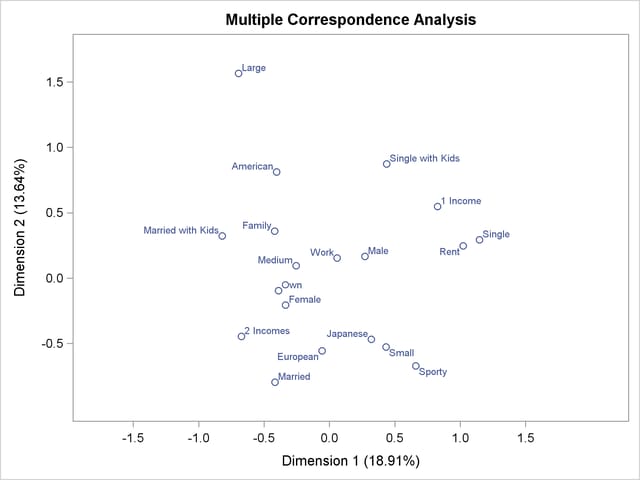
Multiple correspondence analysis locates all the categories in a Euclidean space. The first two dimensions of this space are plotted to examine the associations among the categories. The top-right quadrant of the plot shows that the categories Single, Single with Kids, 1 Income, and Rent are associated. Proceeding clockwise, the categories Sporty, Small, and Japanese are associated. The bottom-left quadrant shows the association between being married, owning your own home, and having two incomes. Having children is associated with owning a large American family auto. Such information could be used in market research to identify target audiences for advertisements.
This interpretation is based on points found in approximately the same direction from the origin and in approximately the same region of the space. Distances between points do not have a straightforward interpretation in multiple correspondence analysis. The geometry of multiple correspondence analysis is not a simple generalization of the geometry of simple correspondence analysis (Greenacre and Hastie; 1987; Greenacre; 1988).
If you want to perform a multiple correspondence analysis and get scores for the individuals, you can specify the BINARY option to analyze the binary table, as in the following statements. In the interest of space, only the first 10 rows of coordinates are printed in Output 31.1.3.
title2 'Binary Table';

* Perform Multiple Correspondence Analysis;
proc corresp data=Cars binary;
   ods select RowCoors;
   tables Origin Size Type Income Home Marital Sex;
run;
| Automobile Owners and Auto Attributes |
| Binary Table |
| The CORRESP Procedure |
| Row Coordinates |
| Dim1 | Dim2 | |
|---|---|---|
| 1 | -0.4093 | 1.0878 |
| 2 | 0.8198 | -0.2221 |
| 3 | -0.2193 | -0.5328 |
| 4 | 0.4382 | 1.1799 |
| 5 | -0.6750 | 0.3600 |
| 6 | -0.1778 | 0.1441 |
| 7 | -0.9375 | 0.6846 |
| 8 | -0.7405 | -0.1539 |
| 9 | -0.3027 | -0.2749 |
| 10 | -0.7263 | -0.0803 |