Overview: SEQTEST Procedure

The purpose of the SEQTEST procedure is to perform interim analyses for clinical trials. Clinical trials are experiments on human beings to demonstrate the efficacy and safety of new drugs or treatments. A simple example is a trial to test the effectiveness of a new drug in humans by comparing the outcomes in a group of patients who receive the new drug with the outcomes in a comparable group of patients who receive a placebo.

A clinical trial is conducted according to a plan called a protocol. A protocol details the objectives of the trial, the data collection process, and the analyses of the data. The protocol contains information such as a null hypothesis and an alternative hypothesis, a test statistic, the probability of a Type I error (incorrectly rejecting the null hypothesis), the probability of a Type II error (incorrectly accepting the null hypothesis), the sample size needed to attain a specified power (probability of correctly rejecting the null hypothesis) of at an alternative reference, and critical values that are associated with the test statistic for hypothesis testing.

In a fixed-sample trial, data about all individuals are first collected and then examined at the end of the study. Most major trials have data safety monitoring boards or data monitoring committees that periodically monitor safety and efficacy data during the trial and recommend that a trial be stopped for safety concerns such as an unacceptable toxicity level. In certain rare situations, the board or committee might even recommend that a trial be stopped for efficacy. In contrast to a fixed-sample trial, a group sequential trial provides for interim analyses before the formal completion of the trial while maintaining the specified overall Type I and Type II error probability levels.

A group sequential trial is most useful in situations where it is important to monitor the trial to prevent unnecessary exposure of patients to an unsafe new drug, or alternatively to a placebo treatment if the new drug shows significant improvement. If a group sequential trial stops early, then it usually requires fewer participants than a corresponding fixed-sample trial.

Thus, in most cases, if a group sequential trial stops early for safety of the new treatment, fewer patients will be exposed to the new treatment than in the fixed-sample trial. Also, if a trial stops early for efficacy of the new treatment, the new treatment will be available sooner than it would be in a fixed-sample trial. Furthermore, if a trial stops early, this can also save time and resources.

A group sequential design provides detailed specifications for a group sequential trial. In addition to the usual specification for a fixed-sample design, it provides the total number of stages (the number of interim stages plus a final stage) and a stopping criterion to reject, to accept, or to either reject or accept the null hypothesis at each interim stage. It also provides critical values and the sample size at each stage for the trial.

At each interim stage, the data collected at the current stage in addition to the data collected at previous stages are analyzed, and statistics such as a maximum likelihood test statistic and its associated standard error are computed. The test statistic is then compared with its corresponding critical values at the stage, and the trial is stopped or continued. If a trial continues to the final stage, the null hypothesis is either rejected or accepted. The critical values for each stage are chosen in such a way to maintain the overall level, the overall level, or both the overall and levels.

Figure 79.1 shows a two-sided symmetric group sequential trial that stops early to reject the null hypothesis that the parameter Trt is zero.

Figure 79.1 Sequential Plot for Two-Sided Test

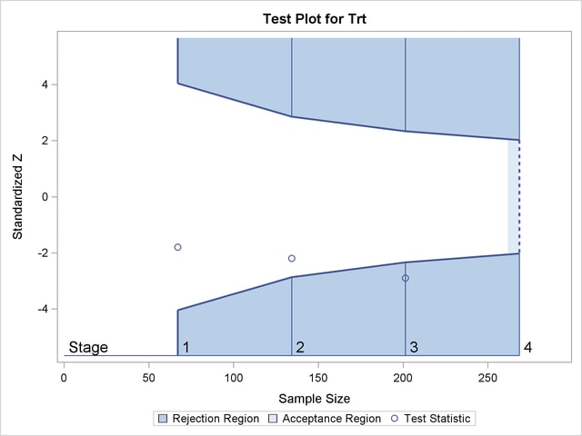
The trial has four stages, which are indicated by vertical lines with accompanying stage numbers. With early stopping to reject the null hypothesis, the lower rejection boundary is constructed by connecting the lower critical values (boundary values) for the stages. Similarly, the upper rejection boundary is constructed by connecting the upper critical values for the stages. The horizontal axis indicates the sample size for the group sequential trial, and the vertical axis indicates the boundary values and test statistics on the standardized scale.

At each interim stage, if the standardized test statistic falls into a rejection region (the darker shaded areas in Figure 79.1), the trial stops and the null hypothesis is rejected. Otherwise, the trial continues to the next stage. At the final stage (stage ), the trial is rejected if falls into a rejection region. Otherwise, the trial is accepted. In Figure 79.1, the test statistic does not fall into the rejection regions for stages and , and so the trial continues to stage . At stage , the test statistic falls into the rejection region, and the null hypothesis is rejected.

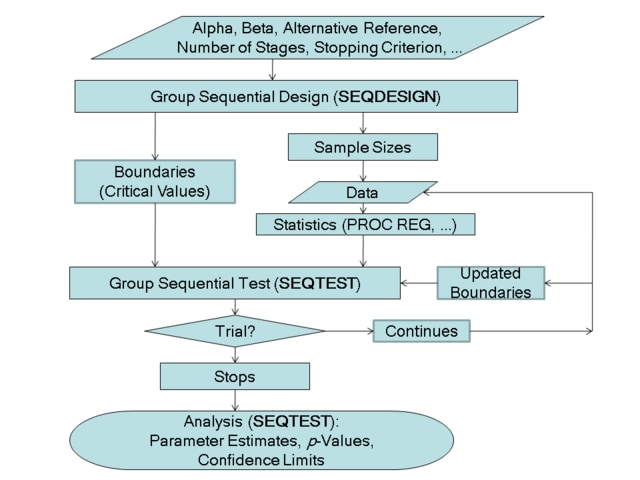
A group sequential trial usually involves six steps:

1. You specify the statistical details of the design, including the null and alternative hypotheses, a test statistic for the hypothesis test, the Type I and II error probabilities, a stopping criterion, the total number of stages, and the relative information level at each stage.

2. You compute the boundary values for the trial based on the specifications in Step 1. You also compute the sample size required at each stage for the specified hypothesis test.

3. At each stage, you collect additional data with the required sample sizes. The data available at each stage include the data collected at previous stages in addition to the data collected at the current stage.

4. At each stage, you analyze the available data with a procedure such as the REG procedure, and you compute the test statistic.

5. At each stage, you compare the test statistic with the corresponding boundary values. You stop the trial to reject or accept the hypothesis, or you continue the trial to the next stage. If you continue the trial to the final stage, you either accept or reject the hypothesis.

6. After the trial stops, you compute parameter estimates, confidence limits for the parameter, and a -value for the hypothesis test.

You use the companion SEQDESIGN procedure at Step to compute the boundary values and required sample sizes for the trial. You use the SEQTEST procedure at Step to compare the test statistic with its boundary values. At stage , the boundary values are derived by using the boundary information tables created by the SEQDESIGN procedure. These boundary information tables are structured for input to the SEQTEST procedure. At each subsequent stage, the boundary values are derived by using the test information tables created by the SEQTEST procedure at the previous stage. These test information tables are also structured for input to the SEQTEST procedure. You also use the SEQTEST procedure at Step to compute parameter estimates, confidence limits, and -values after the trial stops.

Note that for some clinical trials, the information levels are derived from statistics based on individuals specified in the design plan and might not reach the target maximum information level. For example, if an estimate of the variance is used to compute the required sample size for a group sequential trial, the computed variance at each stage might not be the same as the estimated variance. Thus, instead of specifying the number of individuals in the protocol, the information level can be specified. You can then adjust the sample sizes with the updated variance estimates at interim stages to achieve the target maximum information level for the trial (Jennison and Turnbull 2000, p. 295).

The flowchart in Figure 79.2 summarizes the steps in a typical group sequential trial and the relevant SAS procedures.

Figure 79.2 Group Sequential Trial