| The REG Procedure |
Example 74.1 Modeling Salaries of Major League Baseball Players
This example features the use of ODS Graphics in the process of building models by using the REG procedure and highlights the use of fit and influence diagnostics.
The following data set contains salary and performance information for Major League Baseball players who played at least one game in both the 1986 and 1987 seasons, excluding pitchers. The salaries (Sports Illustrated, April 20, 1987) are for the 1987 season and the performance measures are from 1986 (Collier Books, The 1987 Baseball Encyclopedia Update).
 data baseball;
   length name $ 18;
   length team $ 12;
   input name $ 1-18 no_atbat no_hits no_home no_runs no_rbi no_bb yr_major
         cr_atbat cr_hits cr_home cr_runs cr_rbi cr_bb league $
         division $ team $ position $ no_outs no_assts no_error salary;
   logSalary = log10(salary);
   label name="Player's Name"
      no_hits="Hits in 1986"
      no_runs="Runs in 1986"
      no_rbi="RBIs in 1986"
      no_bb="Walks in 1986"
      yr_major="Years in MLB"
      cr_hits="Career Hits"
      salary="1987 Salary in $ Thousands"
      logSalary = "log10(Salary)";
   datalines;
Allanson, Andy       293    66     1    30    29    14
                       1   293    66     1    30    29    14
                    American East Cleveland C 446 33 20 .
Ashby, Alan          315    81     7    24    38    39
                      14  3449   835    69   321   414   375
                    National West Houston C 632 43 10 475
Davis, Alan          479   130    18    66    72    76
                       3  1624   457    63   224   266   263
                    American West Seattle 1B 880 82 14 480
Dawson, Andre        496   141    20    65    78    37
                      11  5628  1575   225   828   838   354
                    National East Montreal RF 200 11 3 500
Galarraga, Andres    321    87    10    39    42    30
                       2   396   101    12    48    46    33
                    National East Montreal 1B 805 40 4 91.5
Griffin, Alfredo     594   169     4    74    51    35
                      11  4408  1133    19   501   336   194

   ... more lines ...

Wilson, Willie       631   170     9    77    44    31
                      11  4908  1457    30   775   357   249
                    American West KansasCity CF 408 4 3 1000
;
Suppose you want to investigate whether you can model the players’ salaries for the 1987 season based on batting statistics for the previous season and lifetime batting performance. Since the variation in salaries is much greater for higher salaries, it is appropriate to apply a log transformation for this analysis. The following statements begin the analysis:
 ods graphics on;

 proc reg data=baseball;
    id name team league;
    model logSalary = no_hits no_runs no_rbi no_bb yr_major cr_hits;
 run;
Output 74.1.1 shows the default output produced by PROC REG. The number of observations table shows that 59 observations are excluded because they have missing values for at least one of the variables used in the analysis. The analysis of variance and parameter estimates tables provide details about the fitted model.
| Number of Observations Read | 322 |
|---|---|
| Number of Observations Used | 263 |
| Number of Observations with Missing Values | 59 |
| Analysis of Variance | |||||
|---|---|---|---|---|---|
| Source | DF | Sum of Squares |
Mean Square |
F Value | Pr > F |
| Model | 6 | 22.92208 | 3.82035 | 60.56 | <.0001 |
| Error | 256 | 16.14954 | 0.06308 | ||
| Corrected Total | 262 | 39.07162 | |||
| Parameter Estimates | ||||||
|---|---|---|---|---|---|---|
| Variable | Label | DF | Parameter Estimate |
Standard Error |
t Value | Pr > |t| |
| Intercept | Intercept | 1 | 1.80065 | 0.05912 | 30.46 | <.0001 |
| no_hits | Hits in 1986 | 1 | 0.00288 | 0.00091244 | 3.15 | 0.0018 |
| no_runs | Runs in 1986 | 1 | 0.00008638 | 0.00173 | 0.05 | 0.9602 |
| no_rbi | RBIs in 1986 | 1 | 0.00054382 | 0.00102 | 0.53 | 0.5947 |
| no_bb | Walks in 1986 | 1 | 0.00292 | 0.00104 | 2.81 | 0.0054 |
| yr_major | Years in MLB | 1 | 0.03087 | 0.00836 | 3.69 | 0.0003 |
| cr_hits | Career Hits | 1 | 0.00010384 | 0.00006328 | 1.64 | 0.1020 |
Before you accept a regression model, it is important to examine influence and fit diagnostics to see whether the model might be unduly influenced by a few observations and whether the data support the assumptions that underlie the linear regression. To facilitate such investigations, you can obtain diagnostic plots by enabling ODS Graphics.
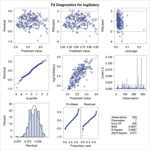
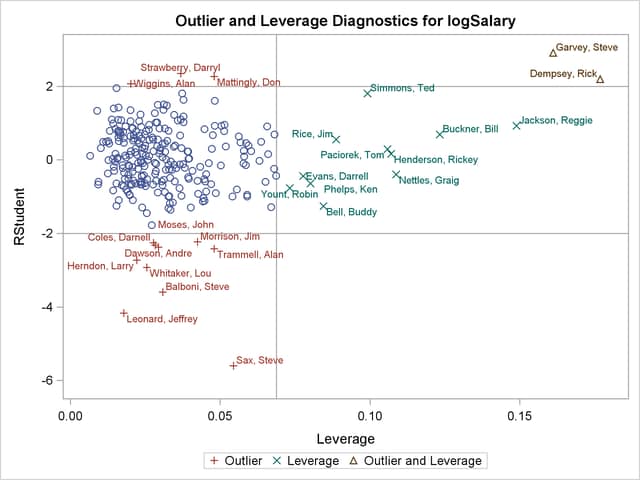
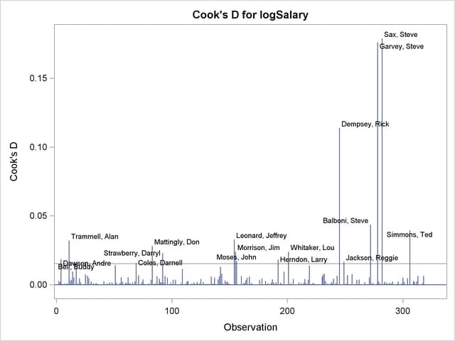
Output 74.1.2 shows a panel of diagnostic plots. The plot of externally studentized residuals (RStudent) by leverage values reveals that there is one observation with very high leverage that might be overly influencing the fit produced. The plot of Cook’s  by observation also indicates two highly influential observations. To investigate further, you can use the PLOTS= option in the PROC REG statement as follows to produce labeled versions of these plots:
 proc reg data=baseball
          plots(only label)=(RStudentByLeverage CooksD);
    id name team league;
    model logSalary = no_hits no_runs no_rbi no_bb yr_major cr_hits;
 run;
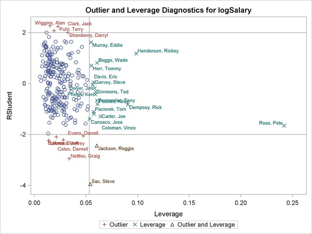
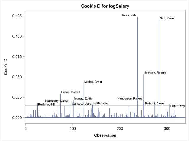
Output 74.1.3 and Output 74.1.4 reveal that Pete Rose is the highly influential observation. You might obtain a better fit to the remaining data if you omit his statistics when building the model.
The following statements use a WHERE statement to omit Pete Rose’s statistics when building the model. An alternative way to do this within PROC REG is to use a REWEIGHT statement. See Reweighting Observations in an Analysis for details about reweighting.
 proc reg data=baseball
          plots=(RStudentByLeverage(label) residuals(smooth));
    where name^="Rose, Pete";
    id name team league;
    model logSalary = no_hits no_runs no_rbi no_bb yr_major cr_hits;
 run;
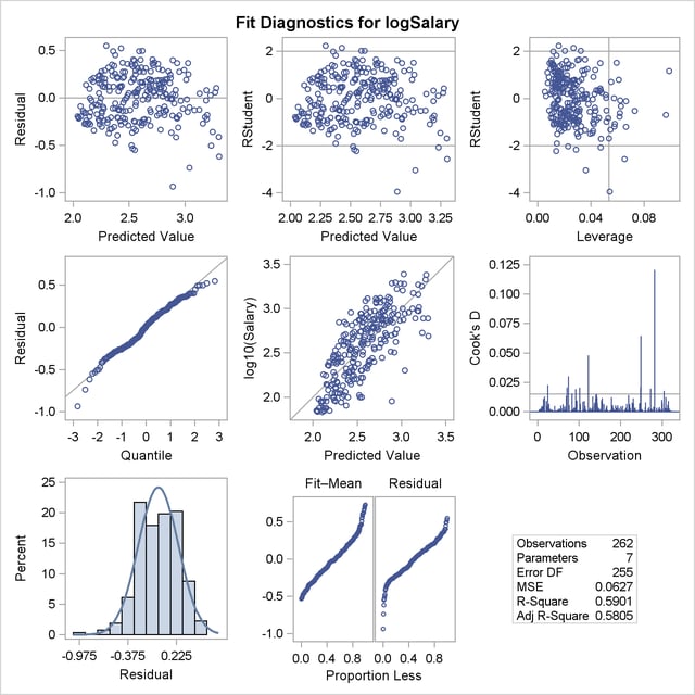
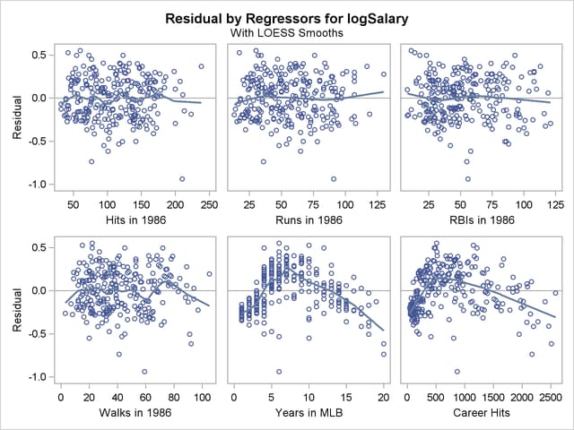
Output 74.1.5 shows the new fit diagnostics panel. You can see that there are still several influential and outlying observations. One possible reason for observing outliers is that the linear model specified is not appropriate to capture the variation in this data. You can often see evidence of an inappropriate model by observing patterns in plots of residuals.
Output 74.1.6 shows plots of the residuals by the regressors in the model. When you specify the RESIDUALS(SMOOTH) suboption of the PLOTS option in the PROC REG statement, a loess fit is overlaid on each of these plots. You can see the same clear pattern in the residual plots for yr_major and cr_hits. Players near the start of their careers and players near the end of their careers get paid less than the model predicts.
You can address this lack of fit by using polynomials of degree 2 for these two variables as shown in the following statements:
 data baseball;
    set baseball(where=(name^="Rose, Pete")) ;
    yr_major2 = yr_major*yr_major;
    cr_hits2  = cr_hits*cr_hits;
 run;

 proc reg data=baseball
       plots=(diagnostics(stats=none) RStudentByLeverage(label)
              CooksD(label) Residuals(smooth)
              DFFITS(label) DFBETAS ObservedByPredicted(label));
    id name team league;
    model logSalary = no_hits no_runs no_rbi no_bb yr_major cr_hits
                      yr_major2 cr_hits2;
 run;
 ods graphics off;
Output 74.1.7 shows the analysis of variance and parameter estimates for this model. Note that the R-square value of  for this model is considerably larger than the R-square value of
  for the initial model shown in Output 74.1.1.
| Analysis of Variance | |||||
|---|---|---|---|---|---|
| Source | DF | Sum of Squares |
Mean Square |
F Value | Pr > F |
| Model | 8 | 30.69367 | 3.83671 | 117.13 | <.0001 |
| Error | 253 | 8.28706 | 0.03276 | ||
| Corrected Total | 261 | 38.98073 | |||
| Parameter Estimates | ||||||
|---|---|---|---|---|---|---|
| Variable | Label | DF | Parameter Estimate |
Standard Error |
t Value | Pr > |t| |
| Intercept | Intercept | 1 | 1.64564 | 0.05030 | 32.72 | <.0001 |
| no_hits | Hits in 1986 | 1 | -0.00005539 | 0.00069200 | -0.08 | 0.9363 |
| no_runs | Runs in 1986 | 1 | 0.00093586 | 0.00125 | 0.75 | 0.4549 |
| no_rbi | RBIs in 1986 | 1 | 0.00187 | 0.00074649 | 2.51 | 0.0127 |
| no_bb | Walks in 1986 | 1 | 0.00218 | 0.00075057 | 2.90 | 0.0040 |
| yr_major | Years in MLB | 1 | 0.10383 | 0.01495 | 6.94 | <.0001 |
| cr_hits | Career Hits | 1 | 0.00073955 | 0.00011970 | 6.18 | <.0001 |
| yr_major2 | 1 | -0.00625 | 0.00071687 | -8.73 | <.0001 | |
| cr_hits2 | 1 | -1.44072E-7 | 4.348471E-8 | -3.31 | 0.0011 | |
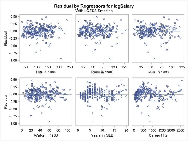
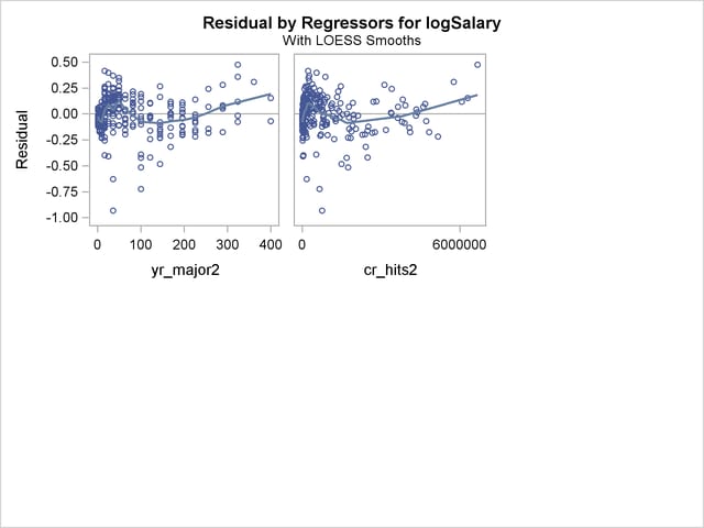
The plots of residuals by regressors in Output 74.1.8 and Output 74.1.9 show that the strong pattern in the plots for cr_majors and cr_hits has been reduced, although there is still some indication of a pattern remaining in these residuals. This suggests that a quadratic function might be insufficient to capture dependence of salary on these regressors.
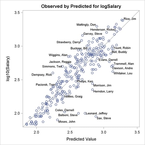
Output 74.1.10 show the diagnostics plots; three of the plots, with points of interest labeled, are shown individually in Output 74.1.11, Output 74.1.12, and Output 74.1.13. The STATS=NONE suboption specified in the PLOTS=DIAGNOSTICS option replaces the inset of statistics with a box plot of the residuals in the fit diagnostics panel. The observed by predicted value plot reveals a reasonably successful model for explaining the variation in salary for most of the players. However, the model tends to overpredict the salaries of several players near the lower end of the salary range. This bias can also be seen in the distribution of the residuals that you can see in the histogram, Q-Q plot, and box plot in Output 74.1.10.
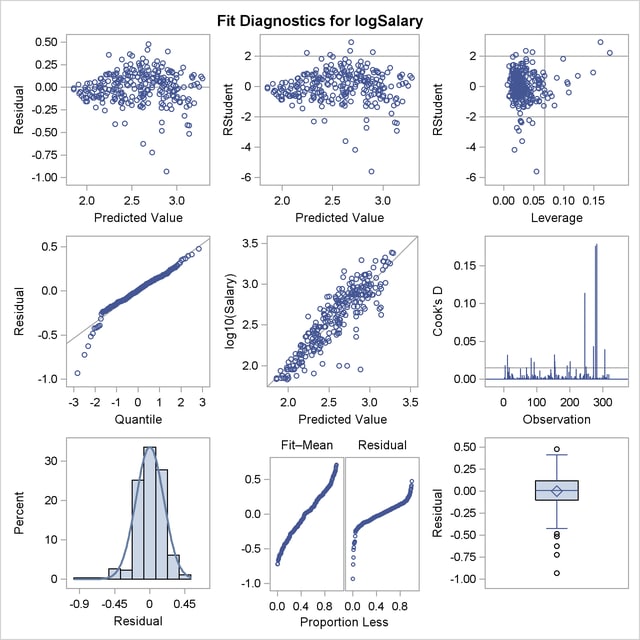
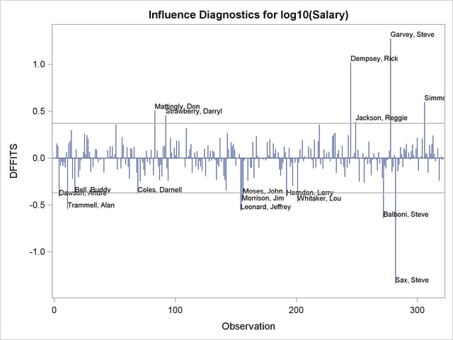
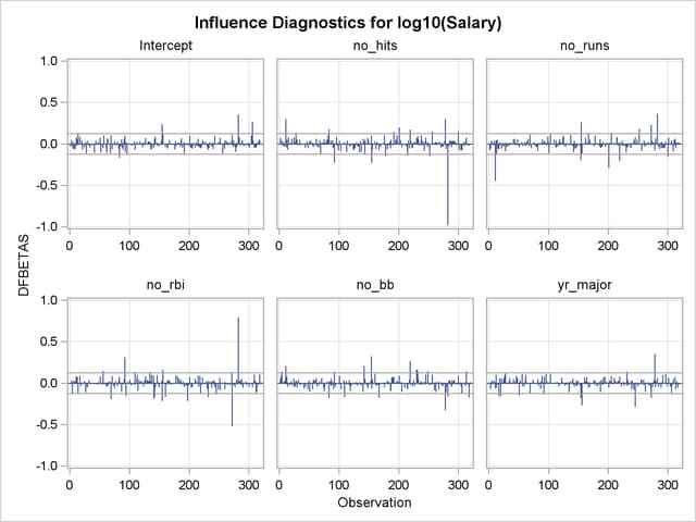
The RStudent by leverage plot in Output 74.1.11 and the Cook’s plot in Output 74.1.13 show that there are still a number of influential observations. By specifying the DFFITS and DFBETAS suboptions of the PLOTS= option, you obtain additional influence diagnostics plots shown in Output 74.1.14 and Output 74.1.15. See Influence Statistics for details about the interpretation DFFITS and DFBETAS statistics.
You can continue this analysis by investigating how the influential observations identified in the various influence plots affect the fit. You can also use PROC ROBUSTREG to obtain a fit that is resistant to the presence of high leverage points and outliers.
Copyright © SAS Institute, Inc. All Rights Reserved.