| The REG Procedure |
| Simple Linear Regression |
Suppose that a response variable  can be predicted by a linear function of a regressor variable
  . You can estimate
  , the intercept, and
  , the slope, in
 |
for the observations  . Fitting this model with the REG procedure requires only the following MODEL statement, where y is the outcome variable and x is the regressor variable.
proc reg;
   model y=x;
run;
For example, you might use regression analysis to find out how well you can predict a child’s weight if you know that child’s height. The following data are from a study of nineteen children. Height and weight are measured for each child.
title 'Simple Linear Regression';
data Class;
   input Name $ Height Weight Age @@;
   datalines;
Alfred  69.0 112.5 14  Alice  56.5  84.0 13  Barbara 65.3  98.0 13
Carol   62.8 102.5 14  Henry  63.5 102.5 14  James   57.3  83.0 12
Jane    59.8  84.5 12  Janet  62.5 112.5 15  Jeffrey 62.5  84.0 13
John    59.0  99.5 12  Joyce  51.3  50.5 11  Judy    64.3  90.0 14
Louise  56.3  77.0 12  Mary   66.5 112.0 15  Philip  72.0 150.0 16
Robert  64.8 128.0 12  Ronald 67.0 133.0 15  Thomas  57.5  85.0 11
William 66.5 112.0 15
;
The equation of interest is
 |
The variable Weight is the response or dependent variable in this equation, and and are the unknown parameters to be estimated. The variable Height is the regressor or independent variable, and  is the unknown error. The following commands invoke the REG procedure and fit this model to the data.
ods graphics on;

proc reg;
   model Weight = Height;
run;

ods graphics off;
Figure 74.1 includes some information concerning model fit.
The  statistic for the overall model is highly significant (=57.076,
  <0.0001), indicating that the model explains a significant portion of the variation in the data.
The degrees of freedom can be used in checking accuracy of the data and model. The model degrees of freedom are one less than the number of parameters to be estimated. This model estimates two parameters, and ; thus, the degrees of freedom should be  . The corrected total degrees of freedom are always one less than the total number of observations in the data set, in this case
  .
.
Several simple statistics follow the ANOVA table. The Root MSE is an estimate of the standard deviation of the error term. The coefficient of variation, or Coeff Var, is a unitless expression of the variation in the data. The R-square and Adj R-square are two statistics used in assessing the fit of the model; values close to 1 indicate a better fit. The R-square of 0.77 indicates that Height accounts for 77% of the variation in Weight.
| Simple Linear Regression |
| Analysis of Variance | |||||
|---|---|---|---|---|---|
| Source | DF | Sum of Squares |
Mean Square |
F Value | Pr > F |
| Model | 1 | 7193.24912 | 7193.24912 | 57.08 | <.0001 |
| Error | 17 | 2142.48772 | 126.02869 | ||
| Corrected Total | 18 | 9335.73684 | |||
| Root MSE | 11.22625 | R-Square | 0.7705 |
|---|---|---|---|
| Dependent Mean | 100.02632 | Adj R-Sq | 0.7570 |
| Coeff Var | 11.22330 |
The "Parameter Estimates" table in Figure 74.2 contains the estimates of and . The table also contains the  statistics and the corresponding -values for testing whether each parameter is significantly different from zero. The -values (
 ,
,  and
and  ,
,  ) indicate that the intercept and Height parameter estimates, respectively, are highly significant.
From the parameter estimates, the fitted model is
 |
If you enable ODS Graphics with an ODS GRAPHICS statement, then PROC REG produces a variety of useful plots. Figure 74.3 shows a plot of the residuals versus the regressor and Figure 74.4 shows a panel of diagnostic plots.
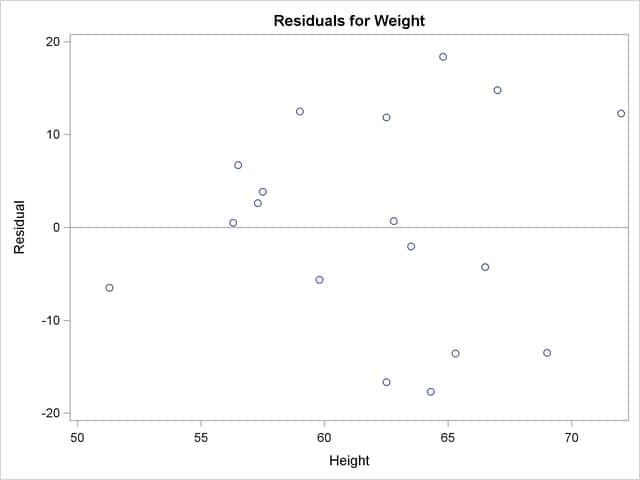
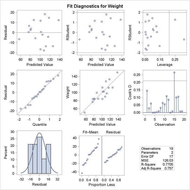
A trend in the residuals would indicate nonconstant variance in the data. The plot of residuals by predicted values in the upper-left corner of the diagnostics panel in Figure 74.4 might indicate a slight trend in the residuals; they appear to increase slightly as the predicted values increase. A fan-shaped trend might indicate the need for a variance-stabilizing transformation. A curved trend (such as a semicircle) might indicate the need for a quadratic term in the model. Since these residuals have no apparent trend, the analysis is considered to be acceptable.
Copyright © SAS Institute, Inc. All Rights Reserved.