| The PHREG Procedure |
Example 64.7 Time-Dependent Repeated Measurements of a Covariate
Repeated determinations can be made during the course of a study of variables thought to be related to survival. Consider an experiment to study the dosing effect of a tumor-promoting agent. Forty-five rodents initially exposed to a carcinogen were randomly assigned to three dose groups. After the first death of an animal, the rodents were examined every week for the number of papillomas. Investigators were interested in determining the effects of dose on the carcinoma incidence after adjusting for the number of papillomas.
The input data set TUMOR consists of the following 19 variables:
ID (subject identification)
Time (survival time of the subject)
Dead (censoring status where 1=dead and 0=censored)
Dose (dose of the tumor-promoting agent)
P1–P15 (number of papillomas at the 15 times that animals died. These 15 death times are weeks 27, 34, 37, 41, 43, 45, 46, 47, 49, 50, 51, 53, 65, 67, and 71. For instance, subject 1 died at week 47; it had no papilloma at week 27, five papillomas at week 34, six at week 37, eight at week 41, and 10 at weeks 43, 45, 46, and 47. For an animal that died before week 71, the number of papillomas is missing for those times beyond its death.)
The following SAS statements create the data set TUMOR:
data Tumor;
   infile datalines missover;
   input ID Time Dead Dose P1-P15;
   label ID='Subject ID';
   datalines;
 1 47 1  1.0  0  5  6  8 10 10 10 10
 2 71 1  1.0  0  0  0  0  0  0  0  0  1  1  1  1 1 1 1
 3 81 0  1.0  0  1  1  1  1  1  1  1  1  1  1  1 1 1 1
 4 81 0  1.0  0  0  0  0  0  0  0  0  0  0  0  0 0 0 0
 5 81 0  1.0  0  0  0  0  0  0  0  0  0  0  0  0 0 0 0
 6 65 1  1.0  0  0  0  1  1  1  1  1  1  1  1  1 1
 7 71 0  1.0  0  0  0  0  0  0  0  0  0  0  0  0 0 0 0
 8 69 0  1.0  0  0  0  0  0  0  0  0  0  0  0  0 0 0
 9 67 1  1.0  0  0  1  1  2  2  2  2  3  3  3  3 3 3
10 81 0  1.0  0  0  0  0  0  0  0  0  0  0  0  0 0 0 0
11 37 1  1.0  9  9  9
12 81 0  1.0  0  0  0  0  0  0  0  0  0  0  0  0 0 0 0
13 77 0  1.0  0  0  0  0  1  1  1  1  1  1  1  1 1 1 1
14 81 0  1.0  0  0  0  0  0  0  0  0  0  0  0  0 0 0 0
15 81 0  1.0  0  0  0  0  0  0  0  0  0  0  0  0 0 0 0
16 54 0  2.5  0  1  1  1  2  2  2  2  2  2  2  2
17 53 0  2.5  0  0  0  0  0  0  0  0  0  0  0  0
18 38 0  2.5  5 13 14
19 54 0  2.5  2  6  6  6  6  6  6  6  6  6  6  6
20 51 1  2.5 15 15 15 16 16 17 17 17 17 17 17
21 47 1  2.5 13 20 20 20 20 20 20 20
22 27 1  2.5 22
23 41 1  2.5  6 13 13 13
24 49 1  2.5  0  3  3  3  3  3  3  3  3
25 53 0  2.5  0  0  1  1  1  1  1  1  1  1  1  1
26 50 1  2.5  0  0  2  3  4  6  6  6  6  6
27 37 1  2.5  3 15 15
28 49 1  2.5  2  3  3  3  3  4  4  4  4
29 46 1  2.5  4  6  7  9  9  9  9
30 48 0  2.5 15 26 26 26 26 26 26 26
31 54 0 10.0 12 14 15 15 15 15 15 15 15 15 15 15
32 37 1 10.0 12 16 17
33 53 1 10.0  3  6  6  6  6  6  6  6  6  6  6  6
34 45 1 10.0  4 12 15 20 20 20
35 53 0 10.0  6 10 13 13 13 15 15 15 15 15 15 20
36 49 1 10.0  0  2  2  2  2  2  2  2  2
37 39 0 10.0  7  8  8
38 27 1 10.0 17
39 49 1 10.0  0  6  9 14 14 14 14 14 14
40 43 1 10.0 14 18 20 20 20
41 28 0 10.0  8
42 34 1 10.0 11 18
43 45 1 10.0 10 12 16 16 16 16
44 37 1 10.0  0  1  1
45 43 1 10.0  9 19 19 19 19
;
The number of papillomas (NPap) for each animal in the study was measured repeatedly over time. One way of handling time-dependent repeated measurements in the PHREG procedure is to use programming statements to capture the appropriate covariate values of the subjects in each risk set. In this example, NPap is a time-dependent explanatory variable with values that are calculated by means of the programming statements shown in the following SAS statements:
proc phreg data=Tumor;
   model Time*Dead(0)=Dose NPap;
   array pp{*} P1-P14;
   array tt{*} t1-t15;
    t1=27;  t2=34;  t3=37;  t4=41;  t5=43;
    t6=45;  t7=46;  t8=47;  t9=49; t10=50;
   t11=51; t12=53; t13=65; t14=67; t15=71;
   if Time <  tt[1]  then NPap=0;
   else if time >= tt[15] then NPap=P15;
   else do i=1 to dim(pp);
      if tt[i] <= Time < tt[i+1] then NPap= pp[i];
   end;
run;
At each death time, the NPap value of each subject in the risk set is recalculated to reflect the actual number of papillomas at the given death time. For instance, subject one in the data set Tumor was in the risk sets at weeks 27 and 34; at week 27, the animal had no papilloma, while at week 34, it had five papillomas. Results of the analysis are shown in Output 64.7.1. After the number of papillomas is adjusted for, the dose effect of the tumor-promoting agent is not statistically significant.
| Model Information | |
|---|---|
| Data Set | WORK.TUMOR |
| Dependent Variable | Time |
| Censoring Variable | Dead |
| Censoring Value(s) | 0 |
| Ties Handling | BRESLOW |
| Summary of the Number of Event and Censored Values |
|||
|---|---|---|---|
| Total | Event | Censored | Percent Censored |
| 45 | 25 | 20 | 44.44 |
| Model Fit Statistics | ||
|---|---|---|
| Criterion | Without Covariates |
With Covariates |
| -2 LOG L | 166.793 | 143.269 |
| AIC | 166.793 | 147.269 |
| SBC | 166.793 | 149.707 |
Another way to handle time-dependent repeated measurements in the PHREG procedure is to use the counting process style of input. Multiple records are created for each subject, one record for each distinct pattern of the time-dependent measurements. Each record contains a T1 value and a T2 value representing the time interval (T1,T2] during which the values of the explanatory variables remain unchanged. Each record also contains the censoring status at T2.
One advantage of using the counting process formulation is that you can easily obtain various residuals and influence statistics that are not available when programming statements are used to compute the values of the time-dependent variables. On the other hand, creating multiple records for the counting process formulation requires extra effort in data manipulation.
Consider a counting process style of input data set named Tumor1. It contains multiple observations for each subject in the data set Tumor. In addition to variables ID, Time, Dead, and Dose, four new variables are generated:
T1 (left endpoint of the risk interval)
T2 (right endpoint of the risk interval)
NPap (number of papillomas in the time interval (T1,T2])
Status (censoring status at T2)
For example, five observations are generated for the rodent that died at week 47 and that had no papilloma at week 27, five papillomas at week 34, six at week 37, eight at week 41, and 10 at weeks 43, 45, 46, and 47. The values of T1, T2, NPap, and Status for these five observations are (0,27,0,0), (27,34,5,0), (34,37,6,0), (37,41,8,0), and (41,47,10,1). Note that the variables ID, Time, and Dead are not needed for the estimation of the regression parameters, but they are useful for plotting the residuals.
The following SAS statements create the data set Tumor1:
  data Tumor1(keep=ID Time Dead Dose T1 T2 NPap Status);
     array pp{*} P1-P14;
     array qq{*} P2-P15;
     array tt{1:15} _temporary_
        (27 34 37 41 43 45 46 47 49 50 51 53 65 67 71);
     set Tumor;
     T1 = 0;
     T2 = 0;
     Status = 0;
     if ( Time = tt[1] ) then do;
        T2 = tt[1];
        NPap = p1;
        Status = Dead;
        output;
     end;
     else do _i_=1 to dim(pp);
        if ( tt[_i_] = Time ) then do;
           T2= Time;
           NPap = pp[_i_] ;
           Status = Dead;
           output;
        end;
        else if (tt[_i_]  < Time ) then do;
           if (pp[_i_]  ^= qq[_i_] ) then do;
              if qq[_i_]  = . then T2= Time;
              else                 T2= tt[_i_] ;
              NPap= pp[_i_] ;
              Status= 0;
              output;
              T1 = T2;
           end;
        end;
     end;
     if ( Time >= tt[15] ) then do;
        T2 = Time;
        NPap = P15;
        Status = Dead;
        output;
     end;
     run;
In the following SAS statements, the counting process MODEL specification is used. The DFBETA statistics are output to a SAS data set named Out1. Note that Out1 contains multiple observations for each subject—that is, one observation for each risk interval (T1,T2].
proc phreg data=Tumor1;
   model (T1,T2)*Status(0)=Dose NPap;
   output out=Out1 resmart=Mart dfbeta=db1-db2;
   id ID Time Dead;
run;
The output from PROC PHREG (not shown) is identical to Output 64.7.1 except for the "Summary of the Number of Event and Censored Values" table. The number of event observations remains unchanged between the two specifications of PROC PHREG, but the number of censored observations differs due to the splitting of each subject’s data into multiple observations for the counting process style of input.
Next, the MEANS procedure sums up the component statistics for each subject and outputs the results to a SAS data set named Out2:
proc means data=Out1 noprint;
   by ID Time Dead;
   var Mart db1-db2;
   output out=Out2 sum=Mart db_Dose db_NPap;
run;
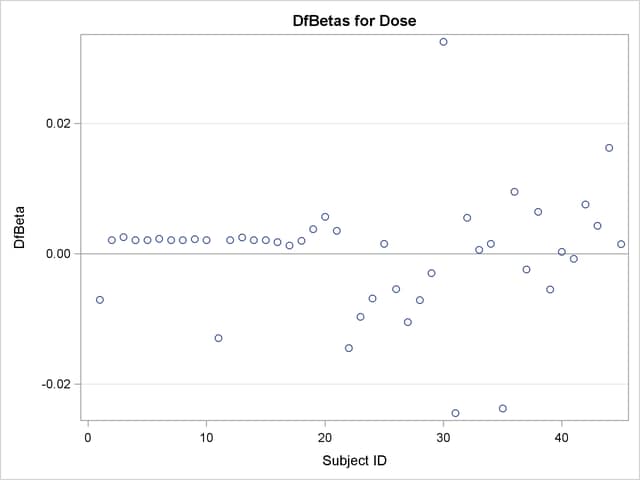
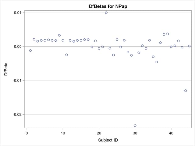
Finally, DFBETA statistics are plotted against subject ID for easy identification of influential points:
title 'DfBetas for Dose';
proc sgplot data=Out2;
   yaxis label="DfBeta" grid;
   refline 0 / axis=y;
   scatter y=db_Dose x=ID;
   run;
title 'DfBetas for NPap';
proc sgplot data=Out2;
   yaxis label="DfBeta" grid;
   refline 0 / axis=y;
   scatter y=db_NPap x=ID;
   run;
The plots of the DFBETA statistics are shown in Output 64.7.2 and Output 64.7.3. Subject 30 appears to have a large influence on both the Dose and NPap coefficients. Subjects 31 and 35 have considerable influences on the DOSE coefficient, while subjects 22 and 44 have rather large influences on the NPap coefficient.


Copyright © SAS Institute, Inc. All Rights Reserved.