| Statistical Graphics Using ODS |
| Partial Least Squares Plots with PROC PLS |
This example is taken from the section Getting Started: PLS Procedure of Chapter 67, The PLS Procedure. The following statements create a SAS data set that contains measurements of biological activity in the Baltic Sea:
data Sample;
   input obsnam $ v1-v27 ls ha dt @@;
   datalines;
EM1   2766 2610 3306 3630 3600 3438 3213 3051 2907 2844 2796
      2787 2760 2754 2670 2520 2310 2100 1917 1755 1602 1467
      1353 1260 1167 1101 1017         3.0110  0.0000   0.00

   ... more lines ...

;
The following statements set the output style to ANALYSIS and run PROC PLS:
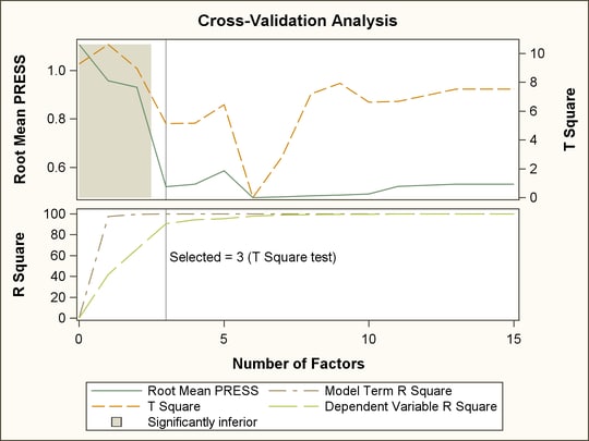
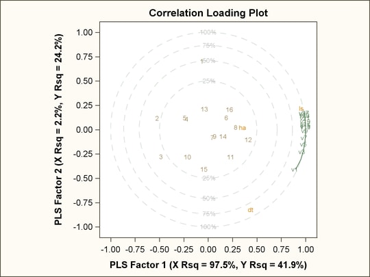
ods listing style=analysis;
ods graphics on;

proc pls data=sample cv=split cvtest(seed=104);
   model ls ha dt = v1-v27;
run;
By default, the procedure produces a plot for the cross validation analysis and a correlation loading plot (see Figure 21.8).
Figure 21.8
Partial Least Squares Results Using the ANALYSIS Style
Copyright © SAS Institute, Inc. All Rights Reserved.