| The MDS Procedure |
Getting Started: MDS Procedure
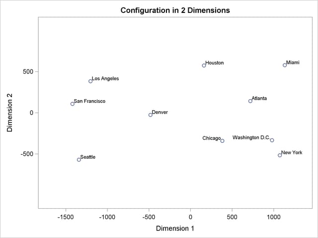
The simplest application of PROC MDS is to reconstruct a map from a table of distances between points on the map (Kruskal and Wish 1978, pp. 7–9). For example, the following DATA step reads a table of flying mileages between 10 U.S. cities:
data city;
   title 'Analysis of Flying Mileages between Ten U.S. Cities';
   input (Atlanta Chicago Denver Houston LosAngeles
          Miami NewYork SanFrancisco Seattle WashingtonDC) (5.)
          @56 City $15.;
   datalines;
    0                                                  Atlanta
  587    0                                             Chicago
 1212  920    0                                        Denver
  701  940  879    0                                   Houston
 1936 1745  831 1374    0                              Los Angeles
  604 1188 1726  968 2339    0                         Miami
  748  713 1631 1420 2451 1092    0                    New York
 2139 1858  949 1645  347 2594 2571    0               San Francisco
 2182 1737 1021 1891  959 2734 2408  678    0          Seattle
  543  597 1494 1220 2300  923  205 2442 2329    0     Washington D.C.
;
Since the flying mileages are very good approximations to Euclidean distance, no transformation is needed to convert distances from the model to data. The analysis can therefore be done at the absolute level of measurement, as displayed in the following PROC MDS step (LEVEL=ABSOLUTE). The following statements produce Figure 53.1 and Figure 53.2:
ods graphics on;

proc mds data=city level=absolute;
   id city;
run;

ods graphics off;
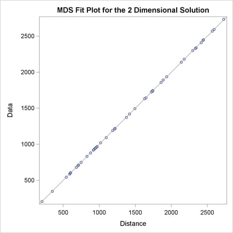
PROC MDS first displays the iteration history. In this example, only one iteration is required. The badness-of-fit criterion 0.001689 indicates that the data fit the model extremely well. You can also see that the fit is excellent in the fit plot in Figure 53.2.
| Analysis of Flying Mileages between Ten U.S. Cities |
| Iteration | Type | Badness- of-Fit Criterion |
Change in Criterion |
Convergence Measure |
|---|---|---|---|---|
| 0 | Initial | 0.003273 | . | 0.8562 |
| 1 | Lev-Mar | 0.001689 | 0.001584 | 0.005128 |
While PROC MDS can recover the relative positions of the cities, it cannot determine absolute location or orientation. In this case, north is toward the bottom of the plot. (See the first plot in Figure 53.2.)
Copyright © SAS Institute, Inc. All Rights Reserved.