| The LIFETEST Procedure |
| Computational Formulas |
Breslow, Fleming-Harrington, and Kaplan-Meier Methods
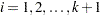
Let  represent the distinct event times. For each
  , let
, let  be the number of surviving units (the size of the risk set) just prior to
  . Let
. Let  be the number of units that fail at , and let
  . If the NOTRUNCATE option is specified in the FREQ statement, , , and
  can be nonintegers.
The Breslow estimate of the survivor function is
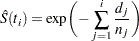 |
Note that the Breslow estimate is the exponentiation of the negative Nelson-Aalen estimate of the cumulative hazard function.
The Fleming-Harrington estimate (Fleming and Harrington; 1984) of the survivor function is
 |
If the frequency values are not integers, the Fleming-Harrington estimate cannot be computed.
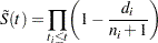
The Kaplan-Meier (product-limit) estimate of the survivor function at is the cumulative product
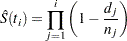 |
Notice that all the estimators are defined to be right continuous; that is, the events at are included in the estimate of  . The corresponding estimate of the standard error is computed using Greenwood’s formula (Kalbfleisch and Prentice; 1980) as
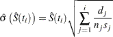 |
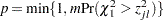
The first quartile (or the 25th percentile) of the survival time is the time beyond which 75% of the subjects in the population under study are expected to survive. It is estimated by
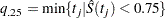 |
If  is exactly equal to 0.75 from
  to
to  , the first quartile is taken to be
  . If it happens that is greater than 0.75 for all values of t, the first quartile cannot be estimated and is represented by a missing value in the printed output.
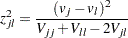
The general formula for estimating the  th percentile point is
 |
The second quartile (the median) and the third quartile of survival times correspond to p=0.5 and p=0.75, respectively.
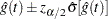
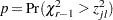
Brookmeyer and Crowley (1982) have constructed the confidence interval for the median survival time based on the confidence interval for the  . The methodology is generalized to construct the confidence interval for the th percentile based on a
  -transformed confidence interval for (Klein and Moeschberger; 1997). You can use the CONFTYPE= option to specify the -transformation. The
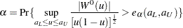
  % confidence interval for the first quantile survival time is the set of all points
  that satisfy
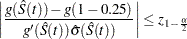 |
where  is the first derivative of
  and
and  is the
  th percentile of the standard normal distribution.
Consider the bone marrow transplant data described in Example 49.2. The following table illustrates the construction of the confidence limits for the first quartile in the ALL group. Values of  that lie between
  =
=  1.965 are highlighted.
Constructing 95% Confidence Limits for the 25th Percentile |
|||||||
|
|||||||
t |
|
|
LINEAR |
LOGLOG |
LOG |
ASINSQRT |
LOGIT |
1 |
0.97368 |
0.025967 |
8.6141 |
2.37831 |
9.7871 |
4.44648 |
2.47903 |
55 |
0.94737 |
0.036224 |
5.4486 |
2.36375 |
6.1098 |
3.60151 |
2.46635 |
74 |
0.92105 |
0.043744 |
3.9103 |
2.16833 |
4.3257 |
2.94398 |
2.25757 |
86 |
0.89474 |
0.049784 |
2.9073 |
1.89961 |
3.1713 |
2.38164 |
1.97023 |
104 |
0.86842 |
0.054836 |
2.1595 |
1.59196 |
2.3217 |
1.87884 |
1.64297 |
107 |
0.84211 |
0.059153 |
1.5571 |
1.26050 |
1.6490 |
1.41733 |
1.29331 |
109 |
0.81579 |
0.062886 |
1.0462 |
0.91307 |
1.0908 |
0.98624 |
0.93069 |
110 |
0.78947 |
0.066135 |
0.5969 |
0.55415 |
0.6123 |
0.57846 |
0.56079 |
122 |
0.73684 |
0.071434 |
-0.1842 |
-0.18808 |
-0.1826 |
-0.18573 |
-0.18728 |
129 |
0.71053 |
0.073570 |
-0.5365 |
-0.56842 |
-0.5222 |
-0.54859 |
-0.56101 |
172 |
0.68421 |
0.075405 |
-0.8725 |
-0.95372 |
-0.8330 |
-0.90178 |
-0.93247 |
192 |
0.65789 |
0.076960 |
-1.1968 |
-1.34341 |
-1.1201 |
-1.24712 |
-1.30048 |
194 |
0.63158 |
0.078252 |
-1.5133 |
-1.73709 |
-1.3870 |
-1.58613 |
-1.66406 |
230 |
0.60412 |
0.079522 |
-1.8345 |
-2.14672 |
-1.6432 |
-1.92995 |
-2.03291 |
276 |
0.57666 |
0.080509 |
-2.1531 |
-2.55898 |
-1.8825 |
-2.26871 |
-2.39408 |
332 |
0.54920 |
0.081223 |
-2.4722 |
-2.97389 |
-2.1070 |
-2.60380 |
-2.74691 |
383 |
0.52174 |
0.081672 |
-2.7948 |
-3.39146 |
-2.3183 |
-2.93646 |
-3.09068 |
418 |
0.49428 |
0.081860 |
-3.1239 |
-3.81166 |
-2.5177 |
-3.26782 |
-3.42460 |
466 |
0.46682 |
0.081788 |
-3.4624 |
-4.23445 |
-2.7062 |
-3.59898 |
-3.74781 |
487 |
0.43936 |
0.081457 |
-3.8136 |
-4.65971 |
-2.8844 |
-3.93103 |
-4.05931 |
526 |
0.41190 |
0.080862 |
-4.1812 |
-5.08726 |
-3.0527 |
-4.26507 |
-4.35795 |
609 |
0.38248 |
0.080260 |
-4.5791 |
-5.52446 |
-3.2091 |
-4.60719 |
-4.64271 |
662 |
0.35306 |
0.079296 |
-5.0059 |
-5.96222 |
-3.3546 |
-4.95358 |
-4.90900 |

Consider the LINEAR transformation where  . The event times that satisfy
 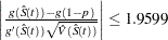 include 107, 109, 110, 122, 129, 172, 192, 194, and 230. The confidence of the interval [107, 230] is less than 95%. Brookmeyer and Crowley (1982) suggest extending the confidence interval to but not including the next event time. As such the 95% confidence interval for the first quartile based on the linear transform is [107, 276). The following table lists the confidence intervals for the various transforms.
95% CI’s for the 25th Percentile |
||
CONFTYPE |
[Lower |
Upper) |
LINEAR |
107 |
276 |
LOGLOG |
86 |
230 |
LOG |
107 |
332 |
ASINSQRT |
104 |
276 |
LOGIT |
104 |
230 |
Sometimes, the confidence limits for the quartiles cannot be estimated. For convenience of explanation, consider the linear transform . If the curve representing the upper confidence limits for the survivor function lies above 0.75, the upper confidence limit for first quartile cannot be estimated. On the other hand, if the curve representing the lower confidence limits for the survivor function lies above 0.75, the lower confidence limit for the quartile cannot be estimated.
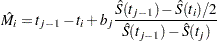
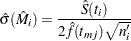
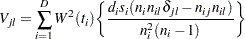
The estimated mean survival time is
 |
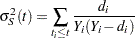
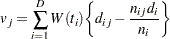
where  is defined to be zero. When the largest observed time is censored, this sum underestimates the mean. The standard error of
  is estimated as
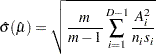 |
where
 |
 |
 |
|||
 |
|
 |
If the largest observed time is not an event, you can use the TIMELIM= option to specify a time limit  and estimate the mean survival time limited to the time and its standard error by replacing
  by
by  with
with  .
.
Nelson-Aalen Estimate of the Cumulative Hazard Function
The Nelson-Aalen cumulative hazard estimator, defined up to the largest observed time on study, is
 |
and its estimated variance is
 |
Life-Table Method
The life-table estimates are computed by counting the numbers of censored and uncensored observations that fall into each of the time intervals  ,
,  , where
  and
and  . Let be the number of units entering the interval , and let be the number of events occurring in the interval. Let
  , and let
  , where
  is the number of units censored in the interval. The effective sample size of the interval is denoted by
  . Let
. Let  denote the midpoint of .
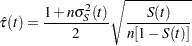
The conditional probability of an event in is estimated by
 |
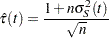
and its estimated standard error is
 |
where  .
.
The estimate of the survival function at is
 |
and its estimated standard error is
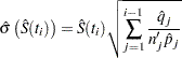 |
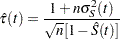
The density function at is estimated by
 |
and its estimated standard error is
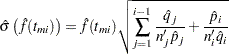 |
The estimated hazard function at is
 |
and its estimated standard error is
 |
Let  be the interval in which
  . The median residual lifetime at is estimated by
 |
and the corresponding standard error is estimated by
 |
Interval Determination
If you want to determine the intervals exactly, use the INTERVALS= option in the PROC LIFETEST statement to specify the interval endpoints. Use the WIDTH= option to specify the width of the intervals, thus indirectly determining the number of intervals. If neither the INTERVALS= option nor the WIDTH= option is specified in the life-table estimation, the number of intervals is determined by the NINTERVAL= option. The width of the time intervals is 2, 5, or 10 times an integer (possibly a negative integer) power of 10. Let  (maximum observed time/number of intervals), and let
  be the largest integer not exceeding
  . Let
. Let  and let
 |
with  being the indicator function. The width is then given by
 |
By default, NINTERVAL=10.
Pointwise Confidence Limits in the OUTSURV= Data Set
Pointwise confidence limits are computed for the survivor function, and for the density function and hazard function when the life-table method is used. Let  be specified by the ALPHA= option. Let
  be the critical value for the standard normal distribution. That is,
 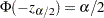 , where
  is the cumulative distribution function of the standard normal random variable.
Survivor Function
When the computation of confidence limits for the survivor function is based on the asymptotic normality of the survival estimator , the approximate confidence interval might include impossible values outside the range [0,1] at extreme values of . This problem can be avoided by applying the asymptotic normality to a transformation of for which the range is unrestricted. In addition, certain transformed confidence intervals for perform better than the usual linear confidence intervals (Borgan and Liestøl; 1990). The CONFTYPE= option enables you to pick one of the following transformations: the log-log function (Kalbfleisch and Prentice; 1980), the arcsine-square root function (Nair; 1984), the logit function (Meeker and Escobar; 1998), the log function, and the linear function.
Let be the transformation that is being applied to the survivor function . By the delta method, the standard error of  is estimated by
 |
where  is the first derivative of the function . The 100(1–)% confidence interval for is given by
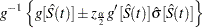 |
where  is the inverse function of .
Arcsine-Square Root Transformation
The estimated variance of  is
is 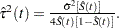 The 100(1–)% confidence interval for is given by
 |
Linear Transformation
This is the same as having no transformation in which is the identity. The 100(1–)% confidence interval for is given by
 |
 is
is  The 100(1–
 is
is 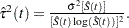 The 100(1–
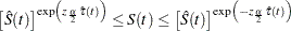
 is
is  The 100(1–
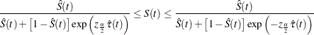
Density and Hazard Functions
For the life-table method, a 100(1–)% confidence interval for hazard function or density function at time is computed as
 |
where  is the estimate of either the hazard function or the density function at time , and
  is the corresponding standard error estimate.
Simultaneous Confidence Intervals for Kaplan-Meier Curves
The pointwise confidence interval for the survivor function is valid for a single fixed time at which the inference is to be made. In some applications, it is of interest to find the upper and lower confidence bands that guarantee, with a given confidence level, that the survivor function falls within the band for all in some interval. Hall and Wellner (1980) and Nair (1984) provide two different approaches for deriving the confidence bands. An excellent review can be found in Klein and Moeschberger (1997). You can use the CONFBAND= option in the SURVIVAL statement to select the confidence bands. The EP confidence band provides confidence bounds that are proportional to the pointwise confidence interval, while those of the HW band are not proportional to the pointwise confidence bounds. The maximum time,  , for the bands can be specified by the BANDMAX= option; the minimum time,
  , can be specified by the BANDMIN= option. Transformations that are used to improve the pointwise confidence intervals can be applied to improve the confidence bands. It might turn out that the upper and lower bounds of the confidence bands are not decreasing in
  , which is contrary to the nonincreasing characteristic of survivor function. Meeker and escobar (1998) suggest making an adjustment so that the bounds do not increase: if the upper bound is increasing on the right, it is made flat from the minimum to ; if the lower bound is increasing from the right, it is made flat from to the maximum. PROC LIFETEST does not make any adjustment for the nondecreasing behavior of the confidence bands in the OUTSURV= data set. However, the adjustment was made in the display of the confidence bands by using ODS Graphics.
For Kaplan-Meier estimation, let  be the
  distinct events times, and at time , there are events. Let
  be the number of individuals who are at risk at time . The variance of , given by the Greenwood formula, is
 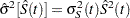 , where
 |
Let  be the time range for the confidence band so that is less than or equal to the largest event time. For the Hall-Wellner band, can be zero, but for the equal-precision band, is greater than or equal to the smallest event time. Let
 |
Let  be a Brownian bridge.
Hall-Wellner Band
The 100(1–)% HW band of Hall and Wellner (1980) is
 |
for all  , where
  is given by
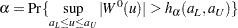 |
The critical values are computed from the results in Chung (1986).
Note that the given confidence band has a formula similar to that of the (linear) pointwise confidence interval, where  and
and  in the former correspond to
  and
and  in the latter, respectively. You can obtain the other transformations (arcsine-square root, log-log, log, and logit) for the confidence bands by replacing and
  in the corresponding pointwise confidence interval formula by and the following , respectively.
Equal-Precision Band
The 100(1–)% EP band of Nair (1984) is
 |
for all  , where
  is given by
 |
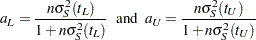
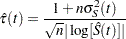
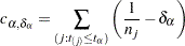
PROC LIFETEST uses the approximation of Miller and Siegmund (1982, Equation 8) to approximate the tail probability in which is obtained by solving  in
in
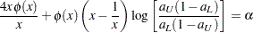 |
where  is the standard normal density function evaluated at . Note that the confidence bounds given are proportional to the pointwise confidence intervals. As a matter of fact, this confidence band and the (linear) pointwise confidence interval have the same formula except for the critical values ( for the pointwise confidence interval and for the band). You can obtain the other transformations (arcsine-square root, log-log, log, and logit) for the confidence bands by replacing by in the formula of the pointwise confidence intervals.
Kernel-Smoothed Hazard Estimate
Kernel-smoothed estimators of the hazard function  are based on the Nelson-Aalen estimator
  and its variance
  . Consider the jumps of and at the event times as follows:
 |
|
 |
|||
 |
 |
 |
where =0.
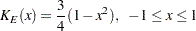
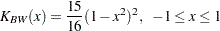
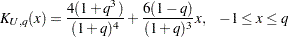
The kernel-smoothed estimator of is a weighted average of  over event times that are within a bandwidth distance of . The weights are controlled by the choice of kernel function,
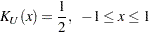
  , defined on the interval [–1,1]. The choices of are as follows:
uniform kernel
Epanechnikov kernel
biweight kernel
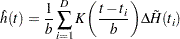
The kernel-smoothed hazard rate estimator is defined for all time points on  . For time points for which
  , the kernel-smoothed estimated of based on the kernel is given by
 |
The variance of  is estimated by
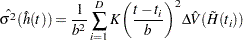 |
For  , the symmetric kernels are replaced by the corresponding asymmetric kernels of Gasser and Müller (1979). Let
  . The modified kernels are as follows:
uniform kernel
Epanechnikov kernel

biweight kernel

For  , let
, let  . The asymmetric kernels for are used with replaced by
  .
.
Using the log transform on the smoothed hazard rate, the 100(1–)% pointwise confidence interval for the smoothed hazard rate is given by
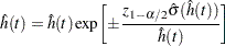 |
where is the 100(1– )th percentile of the standard normal distribution.
Optimal Bandwidth
The following mean integrated squared error (MISE) over the range  and
and  is used as a measure of the global performance of the kernel function estimator
 |
|
 |
|||
 |
 |
 |
The last term is independent of the choice of the kernel and bandwidth and can be ignored when you are looking for the best value of . The first integral can be approximated by using the trapezoid rule by evaluating at a grid of points  . You can specify
  , and
, and  by using the options MISEMIN=, MISEMAX=, and MISENUM=, respectively, of the HAZARD plot. The second integral can be estimated by Ramlau-Hansen (1983a, 1983b) cross-validation estimate
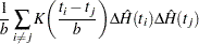 |
Therefore, for a fixed kernel, the optimal bandwidth is the quantity that minimizes
 |
The minimization is carried out by the golden section search algorithm.
Comparison of Two or More Groups of Survival Data
Let be the number of groups. Let  be the underlying survivor function
  th group,
  . The null and alternative hypotheses to be tested are
 for all
versus
 at least one of the ’s is different for some
respectively, where  is the largest observed time.
Likelihood Ratio Test
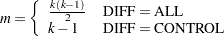
The likelihood ratio test statistic (Lawless; 1982) for test  versus
  assumes that the data in the various samples are exponentially distributed and tests that the scale parameters are equal. The test statistic is computed as
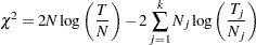 |
where  is the total number of events in the
  th stratum,
  ,
,  is the total time on test in the th stratum, and
  . The approximate probability value is computed by treating
  as having a chi-square distribution with –1 degrees of freedom.
Nonparametric Tests
Let  be the distinct event times in the pooled sample. At time , let
  be a positive weight function, and let
  and
and  be the size of the risk set and the number of events in the th sample, respectively. Let
  ,
,  , and
, and  .
.
The choices of the weight function are given in Table 49.3.
Test |
|
|---|---|
Log-rank |
1.0 |
Wilcoxon |
|
Tarone-Ware |
|
Peto-Peto |
|
Modified Peto-Peto |
|
Harrington-Fleming ( |
|


 ,
, )
) 
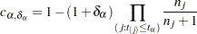
where is the product-limit estimate at for the pooled sample, and  is a survivor function estimate close to given by
 |
Unstratified Tests
The rank statistics (Klein and Moeschberger; 1997, Section 7.3) for testing versus have the form of a -vector  with
with
 |
and the estimated covariance matrix,  , is given by
 |
where  is 1 if
  and 0 otherwise. The term
  can be interpreted as a weighted sum of observed minus expected numbers of failure under the null hypothesis of identical survival curves. The overall test statistic for homogeneity is
  , where
  denotes a generalized inverse of
  . This statistic is treated as having a chi-square distribution with degrees of freedom equal to the rank of for the purposes of computing an approximate probability level.
Stratified Tests
Suppose the test is to be stratified on levels of a set of STRATA variables. Based only on the data of the  th stratum (
 ), let
  be the test statistic (Klein and Moeschberger; 1997, Section 7.5) for the th stratum, and let
  be its covariance matrix. Let
 |
|
 |
|||
 |
|
 |
A global test statistic is constructed as
 |
Under the null hypothesis, the test statistic has a distribution with the same degrees of freedom as the individual test for each stratum.
Multiple-Comparison Adjustments
Let  denote a chi-squared random variable with
  degrees of freedom. Denote
  and as the density function and the cumulative distribution function of a standard normal distribution, respectively. Let
  be the number of comparisons; that is,
 |
For a two-sided test comparing the survival of the th group with that of  th group,
  , the test statistic is
 |
and the raw p-value is
 |
Adjusted p-values for various multiple-comparison adjustments are computed as follows:
- Bonferroni Adjustment
- Dunnett-Hsu Adjustment
With the first group being the control, let
 be the
  matrix of contrasts; that is,
Let
 and
and  be covariance and correlation matrices of
  , respectively; that is,
and

The factor-analytic covariance approximation of Hsu (1992) is to find
 such that
where
 is a diagonal matrix with the th diagonal element being
  and
and 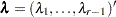 . The adjusted p-value is
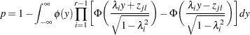
which can be obtained in a DATA step as

- Scheffé Adjustment
 idák Adjustment
- SMM Adjustment
which can also be evaluated in a DATA step as

- Tukey Adjustment

which can also be evaluated in a DATA step as

Trend Tests
Trend tests (Klein and Moeschberger; 1997, Section 7.4) have more power to detect ordered alternatives as
 with at least one inequality
or
 with at least one inequality
Let  be a sequence of scores associated with the samples. The test statistic and its standard error are given by
  and
and  , respectively. Under , the z-score
 |
has, asymptotically, a standard normal distribution. PROC LIFETEST provides both one-tail and two-tail p-values for the test.
Rank Tests for the Association of Survival Time with Covariates
The rank tests for the association of covariates (Kalbfleisch and Prentice; 1980, Chapter 6) are more general cases of the rank tests for homogeneity. In this section, the index is used to label all observations,  , and the indices
  range only over the observations that correspond to events,
  . The ordered event times are denoted as
  , the corresponding vectors of covariates are denoted as
  , and the ordered times, both censored and event times, are denoted as
  .
.
The rank test statistics have the form
 |
where  is the total number of observations,
  are rank scores, which can be either log-rank or Wilcoxon rank scores,
  is 1 if the observation is an event and 0 if the observation is censored, and
  is the vector of covariates in the TEST statement for the th observation. Notice that the scores, , depend on the censoring pattern and that the terms are summed up over all observations.
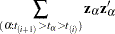
The log-rank scores are
 |
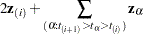
and the Wilcoxon scores are
 |
where  is the number at risk just prior to
  .
.
The estimates used for the covariance matrix of the log-rank statistics are
 |
where  is the corrected sum of squares and crossproducts matrix for the risk set at time ; that is,
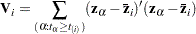 |
where
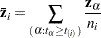 |
The estimate used for the covariance matrix of the Wilcoxon statistics is
 |
where
 |
|
 |
|||
 |
|
 |
|||
 |
|
 |
|||
 |
|
 |
In the case of tied failure times, the statistics  are averaged over the possible orderings of the tied failure times. The covariance matrices are also averaged over the tied failure times. Averaging the covariance matrices over the tied orderings produces functions with appropriate symmetries for the tied observations; however, the actual variances of the statistics would be smaller than the preceding estimates. Unless the proportion of ties is large, it is unlikely that this will be a problem.
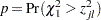
The univariate tests for each covariate are formed from each component of and the corresponding diagonal element of as  . These statistics are treated as coming from a chi-square distribution for calculation of probability values.
The statistic  is computed by sweeping each pivot of the matrix in the order of greatest increase to the statistic. The corresponding sequence of partial statistics is tabulated. Sequential increments for including a given covariate and the corresponding probabilities are also included in the same table. These probabilities are calculated as the tail probabilities of a chi-square distribution with one degree of freedom. Because of the selection process, these probabilities should not be interpreted as p-values.
If desired for data screening purposes, the output data set requested by the OUTTEST= option can be treated as a sum of squares and crossproducts matrix and processed by the REG procedure by using the option METHOD=RSQUARE. Then the sets of variables of a given size can be found that give the largest test statistics. Output 49.1 illustrates this process.
Copyright © SAS Institute, Inc. All Rights Reserved.