| The KRIGE2D Procedure |
Zonal Anisotropy
In zonal anisotropy, the sill (or scale) parameter  is different for different directions. It is not possible to transform such a structure into an isotropic semivariogram. Instead, nesting and geometric anisotropy are used together to approximate zonal anisotropy.
When the scale varies with direction, the lowest scale (that is, the lowest variance) naturally corresponds to the maximum continuity direction. The same direction has the longest range, as also discussed in the section Geometric Anisotropy.
A varying scale with direction can be interpreted as having one or more model components whose individual contributions to the total variance differ with direction. For each such component, its contribution (scale) ranges between zero and a maximum value. This makes it unlikely that you can describe a natural process with a pure zonal model, because doing so would imply zero continuity in the direction of zero contribution; see also Chilès and Delfiner (1999, p. 96).
In a simple case of zonal anisotropy, a model includes one zonal component. The zonal component makes its highest contribution in a direction perpendicular to the maximum continuity direction, and it contributes zero to the maximum continuity direction. This is necessary; otherwise, there would be a direction with a total scale less than the scale in the maximum continuity direction. Following a similar reasoning, the zonal component’s direction of maximum contribution cannot coincide with the one of maximum continuity. In the general case, there can be multiple zonal components, each making its highest contribution in a different direction.
The following describes how to deal with zonal anisotropy in your analysis; see also Goovaerts (1997, p. 96) and Deutsch and Journel (1992, pp. 27–32). If you start with an empirical semivariogram, you can investigate zonal anisotropy by identifying whether a maximum and a minimum scale exist in two specific directions. If they exist, typically these two directions might be perpendicular. Then proceed to identify the zonal component that causes the difference in scale by fitting the empirical semivariogram. You represent zonal component as an additional nested structure in the direction of maximum total scale.
If the minimum and maximum sills are not in perpendicular directions, then you might be seeing the combined effects of multiple zonal components in different directions. In that case you might be able to approximate the continuity behavior by assuming a single zonal component in the direction that is perpendicular to the one of maximum continuity. Alternatively, you might decide to investigate a more elaborate configuration for the model components. In this case, you need to maintain a geometrical anisotropy part across all directions and add zonal components in an appropriate way to match your empirical semivariance in different directions.
After you have a theoretical semivariance model with zonal anisotropy, the next step is to include zonal components in your prediction or simulation analysis. In PROC KRIGE2D you can specify zonal components either explicitly or with the use of results previously saved in item stores produced by the VARIOGRAM procedure.
Specifying a zonal component explicitly in the MODEL statement has the following implications:
The RANGE= parameter for the zonal component refers to the range value in the direction of maximum zonal contribution, unlike the case of ranges specified for nonzonal components that refer to the direction of maximum continuity.
The anisotropy factor
 in the RATIO= parameter for the zonal component should be specified as a large positive value to designate zero contribution in the perpendicular direction.
To explain the previous point, remember that is defined as  . Its value specifies how much to elongate the minor anisotropy axis to make it equal to the major anisotropy axis, in order to transform geometric anisotropy into isotropy. Intuitively, an infinite value makes it impossible for the minor axis to become as large as the major axis. This is equivalent to having a very large major anisotropy axis; hence, it indicates a very large range across the major axis direction. Indeed, you can consider a zero zonal contribution in the major anisotropy axis as a very large range of the zonal component along this direction. The particular range is so large that the zonal component practically never reaches its scale along this direction, and this is interpreted as zero contribution.
In the case where you specify zonal anisotropy by using the contents of an item store, you only need to specify the geometric anisotropy components in the SSEL(MODEL=) option, and the zonal components as suboptions of the SSEL(TYPE=ANIZON) option. Then, the KRIGE2D or SIM2D procedure checks whether the item store contains models that are suitable to use, based on your specifications.
The following two examples illustrate different instances of zonal anisotropy and how to specify the corresponding covariance model parameters in PROC KRIGE2D.
Example 1
The first example shows that if you can model the direction with the highest sill as a nested model, then you can treat the case as a composition of geometric anisotropy and an additional structure that acts only in the direction of the increased sill.
Consider a spatial process in which the fitting of theoretical models in your experimental semivariogram produces a correlation structure like the one shown in Figure 46.14. In the direction  , the covariance model has a single exponential structure
  with range
  and sill
  . In the direction
  , the covariance model
  has two nested structures: an exponential structure with range
  and sill
  and a spherical structure with range
  and sill
  .
.
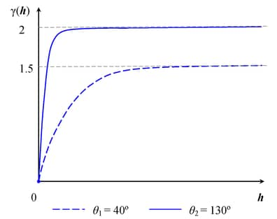
The total sill in the direction  of highest variance is the sum of the nested structures’ sills
  . You can consider that your process is characterized by a geometrically anisotropic exponential structure with common sill
  across all directions and major axis range , and by a spherical structure which is a zonal anisotropy component that contributes only in the direction. Based on the remarks in this section, the RATIO= parameter for the exponential structure is
  , whereas for the spherical structure you choose a large value, such as
  .
.
Then, you can approximate this structure in PROC KRIGE2D by specifying the two structures with the following MODEL statement:
MODEL FORM=(EXP,SPH) RANGE=(2,1) SCALE=(1.5,0.5)
      ANGLE=(40,130) RATIO=(0.25,1E8);
You can handle more elaborate cases in a similar way, where the covariance models in different directions might all be nested models. Your goal is to model the continuity by starting with a sum of isotropic or geometrically anisotropic structures whose total sill is the lowest sill in all directions. Then, in each of the directions with higher sills you add a zonal anisotropy component to the corresponding sum to compensate for the increased variability in that direction.
Example 2
The second example provides important perspective about the physics of zonal anisotropy analysis. It is an extreme case of the general guidelines for zonal anisotropy. You examine what happens when each of the directions is modeled with a single-form, non-nested model, and the sills for these models are clearly different.
Consider a spatial process with a continuity description almost identical to the one in the previous example. In the direction , the covariance model has again a single exponential structure with range and sill . However, this time in the direction you have fit the experimental semivariogram by using a single exponential structure  with range
  and sill
  . These models are shown in Figure 46.15.
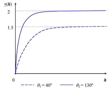
In this case you have a simplified situation with a single covariance structure in each direction, and the two structures have different scale parameter values. This is a case of zonal anisotropy in which all directions have no shared component. Hence, you have a case with two pure zonal components, where both structures can be practically approximated by specifying two models with large RATIO= values. You could then use the following MODEL statement in PROC KRIGE2D to describe the covariance in this example:
MODEL FORM=(EXP,EXP) RANGE=(2,1) SCALE=(1.5,2)
      ANGLE=(40,130) RATIO=(1E8,1E8);
The semivariogram of the specified model is accurately shown in Figure 46.15, because the angles  and are perpendicular and each component has a contribution to all directions except for the one that is perpendicular to its angle. In the general case, and might not be perpendicular; hence the maximum and minimum scale values can be different from those displayed in Figure 46.15.
In general, avoid configurations with pure zonal components. Correlation models with pure zonal components might imply zero continuity along some direction, which is a very unlikely occurrence in natural processes. For that reason, in similar cases try to use the analysis illustrated in the previous example. In particular, try to model the highest sill direction as a nested structure (such that it contains a geometrical anisotropy component whose cumulative sill is equal to the lower sill) and a zonal anisotropy component that accounts for the sill difference.
Copyright © SAS Institute, Inc. All Rights Reserved.