Getting Started: KDE Procedure

The following example illustrates the basic features of PROC KDE. Assume that 1000 observations are simulated from a bivariate normal density with means , variances , and covariance . The SAS DATA step to accomplish this is as follows:

data bivnormal;
   seed = 1283470;
   do i = 1 to 1000;
      z1 = rannor(seed);
      z2 = rannor(seed);
      z3 = rannor(seed);
      x = 3*z1+z2;
      y = 3*z1+z3;
      output;
   end;
   drop seed;
run;

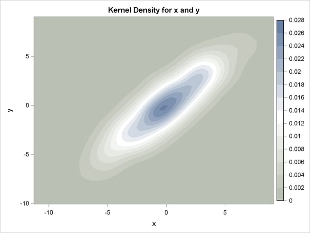
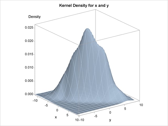
The following statements request a bivariate kernel density estimate for the variables x and y, with contour and surface plots:

ods graphics on;
proc kde data=bivnormal; 
   bivar x y / plots=(contour surface);
run;
ods graphics off;

The contour plot and the surface plot of the estimate are displayed in Figure 45.1 and Figure 45.2, respectively. Note that the correlation of in the original data results in oval-shaped contours. These graphs are produced by specifying the ODS GRAPHICS statement prior to the PROC statement and the PLOTS= option in the BIVAR statement. For general information about ODS Graphics, see Chapter 21, Statistical Graphics Using ODS. For specific information about the graphics available in the KDE procedure, see the section ODS Graphics.

Figure 45.1 Contour Plot of Estimated Density

Figure 45.2 Surface Plot of Estimated Density

The default output tables for this analysis are shown in Figure 45.3.

The "Inputs" table lists basic information about the density fit, including the input data set, the number of observations, and the variables. The bandwidth method is the technique used to select the amount of smoothing in the estimate. A simple normal reference rule is used for bivariate smoothing.

The "Controls" table lists the primary numbers controlling the kernel density fit. Here a grid is fit to the entire range of the data, and no adjustment is made to the default bandwidth.