| Introduction to Categorical Data Analysis Procedures |
| Simple Random Sampling: One Population |
Suppose you take a simple random sample of 100 people and ask each person the following question, "Of the three colors red, blue, and green, which is your favorite?" You then tabulate the results in a frequency table as shown in Table 8.1.
Favorite Color |
||||
|---|---|---|---|---|
Red |
Blue |
Green |
Total |
|
Frequency |
52 |
31 |
17 |
100 |
Proportion |
0.52 |
0.31 |
0.17 |
1.00 |
In the population you are sampling, you assume there is an unknown probability that a population member, selected at random, would choose any given color. In order to estimate that probability, you use the sample proportion
 |
where  is the frequency of the
  th response and
  is the total frequency.
Because of the random variation inherent in any random sample, the frequencies have a probability distribution representing their relative frequency of occurrence in a hypothetical series of samples. For a simple random sample, the distribution of frequencies for a frequency table with three levels is as follows. The probability that the first frequency is  , the second frequency is
  , and the third is
  , is given by
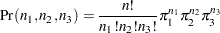 |
where  is the true probability of observing the th response level in the population.
This distribution, called the multinomial distribution, can be generalized to any number of response levels. The special case of two response levels is called the binomial distribution.
Simple random sampling is the type of sampling required by the (non-survey) modeling procedures when there is one population. The modeling procedures use the multinomial distribution to estimate a probability vector and its covariance matrix. If the sample size is sufficiently large, then the probability vector is approximately normally distributed as a result of central limit theory. This result is used to compute appropriate test statistics for the specified statistical model.
Copyright © SAS Institute, Inc. All Rights Reserved.