| The INBREED Procedure |
| Computational Details |
This section describes the rules that the INBREED procedure uses to compute the covariance and inbreeding coefficients. Each computational rule is explained by an example referring to the fictitious population introduced in the section Getting Started: INBREED Procedure.
Coancestry (or Kinship Coefficient)
To calculate the inbreeding coefficient and the covariance coefficients, use the degree of relationship by descent between the two parents, which is called coancestry or kinship coefficient (Falconer and Mackay; 1996, p.85), or coefficient of parentage (Kempthorne; 1957, p.73). Denote the coancestry between individuals X and Y by  . For information on how to calculate the coancestries among a population, see the section Calculation of Coancestry.
Covariance Coefficient (or Coefficient of Relationship)
The covariance coefficient between individuals X and Y is defined by
 |
where is the coancestry between X and Y. The covariance coefficient is sometimes called the coefficient of relationship or the theoretical correlation (Falconer and Mackay (1996, p.153); Crow and Kimura (1970, p.134)). If a covariance coefficient cannot be calculated from the individuals in the population, it is assigned to an initial value. The initial value is set to 0 if the INIT= option is not specified or to cov if INIT=cov. Therefore, the corresponding initial coancestry is set to 0 if the INIT= option is not specified or to  cov if INIT=cov.
Inbreeding Coefficients
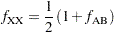
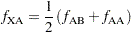
The inbreeding coefficient of an individual is the probability that the pair of alleles carried by the gametes that produced it are identical by descent (Falconer and Mackay (1996, Chapter 5), Kempthorne (1957, Chapter 5)). For individual X, denote its inbreeding coefficient by  . The inbreeding coefficient of an individual is equal to the coancestry between its parents. For example, if X has parents A and B, then the inbreeding coefficient of X is
 |
Calculation of Coancestry
Given individuals X and Y, assume that X has parents A and B and that Y has parents C and D. For nonoverlapping generations, the basic rule to calculate the coancestry between X and Y is given by the following formula (Falconer and Mackay; 1996, p.86):
 |
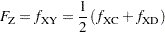
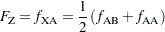
And the inbreeding coefficient for an offspring of X and Y, called Z, is the coancestry between X and Y:
 |
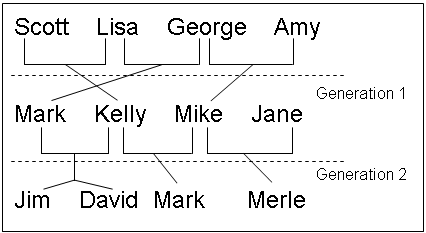
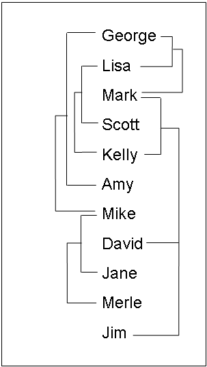
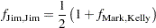
For example, in Figure 44.4, ‘Jim’ and ‘Mark’ from Generation 2 are progenies of ‘Mark’ and ‘Kelly’ and of ‘Mike’ and ‘Kelly’ from Generation 1, respectively. The coancestry between ‘Jim’ and ‘Mark’ is
 |
From the covariance matrix for Generation=1 in Figure 44.4 and the relationship that coancestry is half of the covariance coefficient,
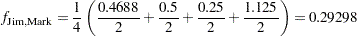 |
For overlapping generations, if X is older than Y, then the basic rule can be simplified to
 |
That is, the coancestry between X and Y is the average of coancestries between older X with younger Y’s parents. For example, in Figure 44.5, the coancestry between ‘Kelly’ and ‘David’ is
 |
This is so because ‘Kelly’ is defined before ‘David’; therefore, ‘Kelly’ is not younger than ‘David’, and the parents of ‘David’ are ‘Mark’ and ‘Kelly’. The covariance coefficient values Cov(Kelly,Mark) and Cov(Kelly,Kelly) from the matrix in Figure 44.5 yield that the coancestry between ‘Kelly’ and ‘David’ is
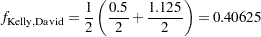 |
The numerical values for some initial coancestries must be known in order to use these rule. Either the parents of the first generation have to be unrelated, with  if the INIT= option is not specified in the PROC statement, or their coancestries must have an initial value of cov, where cov is set by the INIT= option. Then the subsequent coancestries among their progenies and the inbreeding coefficients of their progenies in the rest of the generations are calculated by using these initial values.
Special rules need to be considered in the calculations of coancestries for the following cases.
Self-Mating
The coancestry for an individual X with itself,  , is the inbreeding coefficient of a progeny that is produced by self-mating. The relationship between the inbreeding coefficient and the coancestry for self-mating is
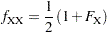 |
The inbreeding coefficient can be replaced by the coancestry between X’s parents A and B,  , if A and B are in the population:
 |
If X’s parents are not in the population, then is replaced by the initial value cov if cov is set by the INIT= option, or is replaced by 0 if the INIT= option is not specified. For example, the coancestry of ‘Jim’ with himself is
 |
where ‘Mark’ and ‘Kelly’ are the parents of ‘Jim’. Since the covariance coefficient Cov(Mark,Kelly) is 0.5 in Figure 44.5 and also in the covariance matrix for GENDER=1 in Figure 44.4, the coancestry of ‘Jim’ with himself is
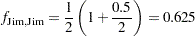 |
When INIT=0.25, then the coancestry of ‘Jane’ with herself is
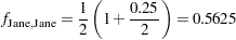 |
because ‘Jane’ is not an offspring in the population.
Offspring and Parent Mating
Assuming that X’s parents are A and B, the coancestry between X and A is
 |
The inbreeding coefficient for an offspring of X and A, denoted by Z, is
 |
For example, ‘Mark’ is an offspring of ‘George’ and ‘Lisa’, so the coancestry between ‘Mark’ and ‘Lisa’ is
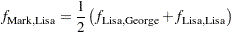 |
From the covariance coefficient matrix in Figure 44.5,  ,
,  so that
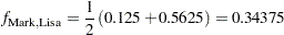 |
Thus, the inbreeding coefficient for an offspring of ‘Mark’ and ‘Lisa’ is 0.34375.
Full Sibs Mating
This is a special case for the basic rule given at the beginning of the section Calculation of Coancestry. If X and Y are full sibs with same parents A and B, then the coancestry between X and Y is
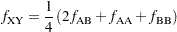 |
and the inbreeding coefficient for an offspring of A and B, denoted by Z, is
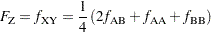 |
For example, ‘David’ and ‘Jim’ are full sibs with parents ‘Mark’ and ‘Kelly’, so the coancestry between ‘David’ and ‘Jim’ is
 |
Since the coancestry is half of the covariance coefficient, from the covariance matrix in Figure 44.5,
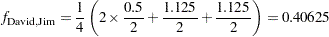 |
Unknown or Missing Parents
When individuals or their parents are unknown in the population, their coancestries are assigned by the value cov if cov is set by the INIT= option or by the value 0 if the INIT= option is not specified. That is, if either A or B is unknown, then
 |
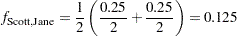
For example, ‘Jane’ is not in the population, and since ‘Jane’ is assumed to be defined just before the observation at which ‘Jane’ appears as a parent (that is, between observations 4 and 5), then ‘Jane’ is not older than ‘Scott’. The coancestry between ‘Jane’ and ‘Scott’ is then obtained by using the simplified basic rule (see the section Calculation of Coancestry):
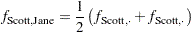 |
Here, dots ( ) indicate Jane’s unknown parents. Therefore,
  is replaced by cov, where cov is set by the INIT= option. If INIT=0.25, then
 |
For a more detailed discussion on the calculation of coancestries, inbreeding coefficients, and covariance coefficients, refer to Falconer and Mackay (1996), Kempthorne (1957), and Crow and Kimura (1970).
Copyright © SAS Institute, Inc. All Rights Reserved.