| The GLIMMIX Procedure |
Pseudo-likelihood Estimation Based on Linearization
The Pseudo-model
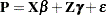
Recall from the section Notation for the Generalized Linear Mixed Model that
 |
where  and
and 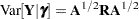 . Following Wolfinger and O’Connell (1993), a first-order Taylor series of
  about
about  and
and  yields
 |
where
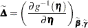 |
is a diagonal matrix of derivatives of the conditional mean evaluated at the expansion locus. Rearranging terms yields the expression
 |
The left side is the expected value, conditional on  , of
, of
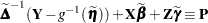 |
and
 |
You can thus consider the model
 |
which is a linear mixed model with pseudo-response  , fixed effects
  , random effects , and
 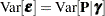 .
.
Objective Functions
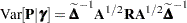
Now define
 |
as the marginal variance in the linear mixed pseudo-model, where  is the
  parameter vector containing all unknowns in
  and
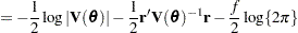
and  . Based on this linearized model, an objective function can be defined, assuming that the distribution of is known. The GLIMMIX procedure assumes that
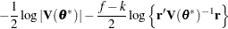
  has a normal distribution. The maximum log pseudo-likelihood (MxPL) and restricted log pseudo-likelihood (RxPL) for are then
 |
 |
|||
 |
 |
with  .
.  denotes the sum of the frequencies used in the analysis, and
  denotes the rank of
  . The fixed-effects parameters are profiled from these expressions. The parameters in are estimated by the optimization techniques specified in the NLOPTIONS statement. The objective function for minimization is
  or
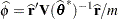
or  . At convergence, the profiled parameters are estimated and the random effects are predicted as
 |
 |
|||
 |
 |
With these statistics, the pseudo-response and error weights of the linearized model are recomputed and the objective function is minimized again. The predictors  are the estimated BLUPs in the approximated linear model. This process continues until the relative change between parameter estimates at two successive (outer) iterations is sufficiently small. See the PCONV= option in the PROC GLIMMIX statement for the computational details about how the GLIMMIX procedure compares parameter estimates across optimizations.
If the conditional distribution contains a scale parameter  (Table 38.15), the GLIMMIX procedure profiles this parameter in GLMMs from the log pseudo-likelihoods as well. To this end define
 |
where  is the covariance parameter vector with
  elements. The matrices
  and
and  are appropriately reparameterized versions of
  and
and  . For example, if has a variance component structure and
  , then contains ratios of the variance components and
  , and
, and  . The solution for
  is
is
 |
where  for MxPL and
  for RxPL. Substitution into the previous functions yields the profiled log pseudo-likelihoods,
 |
 |
|||
 |
 |
|||
 |
 |
Profiling of can be suppressed with the NOPROFILE option in the PROC GLIMMIX statement.
Where possible, the objective function, its gradient, and its Hessian employ the sweep-based W-transformation (Hemmerle and Hartley 1973; Goodnight 1979; Goodnight and Hemmerle 1979). Further details about the minimization process in the general linear mixed model can be found in Wolfinger, Tobias, and Sall (1994).
Estimated Precision of Estimates
The GLIMMIX procedure produces estimates of the variability of  ,
,  , and estimates of the prediction variability for ,
  . Denote as
  the matrix
 |
where all components on the right side are evaluated at the converged estimates. The mixed model equations (Henderson 1984) in the linear mixed (pseudo-)model are then
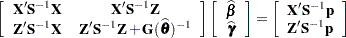 |
and
 |
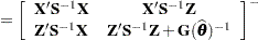 |
|||
|
 |
is the approximate estimated variance-covariance matrix of  . Here,
  and
and 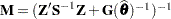 .
.
The square roots of the diagonal elements of  are reported in the Standard Error column of the "Parameter Estimates" table. This table is produced with the SOLUTION option in the MODEL statement. The prediction standard errors of the random-effects solutions are reported in the Std Err Pred column of the "Solution for Random Effects" table. This table is produced with the SOLUTION option in the RANDOM statement.
As a cautionary note,  tends to underestimate the true sampling variability of [
 , because no account is made for the uncertainty in estimating and . Although inflation factors have been proposed (Kackar and Harville 1984; Kass and Steffey 1989; Prasad and Rao 1990), they tend to be small for data sets that are fairly well balanced. PROC GLIMMIX does not compute any inflation factors by default. The DDFM=KENWARDROGER option in the MODEL statement prompts PROC GLIMMIX to compute a specific inflation factor (Kenward and Roger 1997), along with Satterthwaite-based degrees of freedom.
If  is singular, or if you use the CHOL option of the PROC GLIMMIX statement, the mixed model equations are modified as follows. Let
  denote the lower triangular matrix so that
  . PROC GLIMMIX then solves the equations
 |
and transforms  and a generalized inverse of the left-side coefficient matrix by using .
The asymptotic covariance matrix of the covariance parameter estimator is computed based on the observed or expected Hessian matrix of the optimization procedure. Consider first the case where the scale parameter is not present or not profiled. Because is profiled from the pseudo-likelihood, the objective function for minimization is 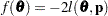 for METHOD=MSPL and METHOD=MMPL and
  for METHOD=RSPL and METHOD=RMPL. Denote the observed Hessian (second derivative) matrix as
 |
The GLIMMIX procedure computes the variance of by default as  . If the Hessian is not positive definite, a sweep-based generalized inverse is used instead. When the EXPHESSIAN option of the PROC GLIMMIX statement is used, or when the procedure is in scoring mode at convergence (see the SCORING option in the PROC GLIMMIX statement), the observed Hessian is replaced with an approximated expected Hessian matrix in these calculations.
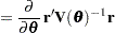
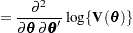
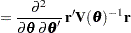
Following Wolfinger, Tobias, and Sall (1994), define the following components of the gradient and Hessian in the optimization:
 |
 |
|||
 |
 |
|||
 |
 |
|||
 |
 |
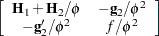
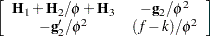
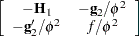
Table 38.18 gives expressions for the Hessian matrix  depending on estimation method, profiling, and scoring.
Profiling |
Scoring |
MxPL |
RxPL |
|---|---|---|---|
No |
No |
|
|
No |
Yes |
|
|
No |
Mod. |
|
|
Yes |
No |
|
|
Yes |
Yes |
|
|
Yes |
Mod. |
|
|


The "Mod." expressions for the Hessian under scoring in RxPL estimation refer to a modified scoring method. In some cases, the modification leads to faster convergence than the standard scoring algorithm. The modification is requested with the SCOREMOD option in the PROC GLIMMIX statement.
Finally, in the case of a profiled scale parameter , the Hessian for the  parameterization is converted into that for the parameterization as
 |
where
 |
Subject-Specific and Population-Averaged (Marginal) Expansions
There are two basic choices for the expansion locus of the linearization. A subject-specific (SS) expansion uses
 |
which are the current estimates of the fixed effects and estimated BLUPs. The population-averaged (PA) expansion expands about the same fixed effects and the expected value of the random effects
 |
To recompute the pseudo-response and weights in the SS expansion, the BLUPs must be computed every time the objective function in the linear mixed model is maximized. The PA expansion does not require any BLUPs. The four pseudo-likelihood methods implemented in the GLIMMIX procedure are the  factorial combination between two expansion loci and residual versus maximum pseudo-likelihood estimation. The following table shows the combination and the corresponding values of the METHOD= option (PROC GLIMMIX statement); METHOD=RSPL is the default.
Type of |
Expansion Locus |
|
|---|---|---|
PL |
|
E |
residual |
RSPL |
RMPL |
maximum |
MSPL |
MMPL |

Copyright © SAS Institute, Inc. All Rights Reserved.