| The GENMOD Procedure |
| Bayesian Analysis of a Linear Regression Model |
Neter et al. (1996) describe a study of 54 patients undergoing a certain kind of liver operation in a surgical unit. The data set Surg contains survival time and certain covariates for each patient. Observations for the first 20 patients in the data set Surg are shown in Figure 37.7.
| Obs | x1 | x2 | x3 | x4 | y | logy | Logx1 |
|---|---|---|---|---|---|---|---|
| 1 | 6.7 | 62 | 81 | 2.59 | 200 | 2.3010 | 1.90211 |
| 2 | 5.1 | 59 | 66 | 1.70 | 101 | 2.0043 | 1.62924 |
| 3 | 7.4 | 57 | 83 | 2.16 | 204 | 2.3096 | 2.00148 |
| 4 | 6.5 | 73 | 41 | 2.01 | 101 | 2.0043 | 1.87180 |
| 5 | 7.8 | 65 | 115 | 4.30 | 509 | 2.7067 | 2.05412 |
| 6 | 5.8 | 38 | 72 | 1.42 | 80 | 1.9031 | 1.75786 |
| 7 | 5.7 | 46 | 63 | 1.91 | 80 | 1.9031 | 1.74047 |
| 8 | 3.7 | 68 | 81 | 2.57 | 127 | 2.1038 | 1.30833 |
| 9 | 6.0 | 67 | 93 | 2.50 | 202 | 2.3054 | 1.79176 |
| 10 | 3.7 | 76 | 94 | 2.40 | 203 | 2.3075 | 1.30833 |
| 11 | 6.3 | 84 | 83 | 4.13 | 329 | 2.5172 | 1.84055 |
| 12 | 6.7 | 51 | 43 | 1.86 | 65 | 1.8129 | 1.90211 |
| 13 | 5.8 | 96 | 114 | 3.95 | 830 | 2.9191 | 1.75786 |
| 14 | 5.8 | 83 | 88 | 3.95 | 330 | 2.5185 | 1.75786 |
| 15 | 7.7 | 62 | 67 | 3.40 | 168 | 2.2253 | 2.04122 |
| 16 | 7.4 | 74 | 68 | 2.40 | 217 | 2.3365 | 2.00148 |
| 17 | 6.0 | 85 | 28 | 2.98 | 87 | 1.9395 | 1.79176 |
| 18 | 3.7 | 51 | 41 | 1.55 | 34 | 1.5315 | 1.30833 |
| 19 | 7.3 | 68 | 74 | 3.56 | 215 | 2.3324 | 1.98787 |
| 20 | 5.6 | 57 | 87 | 3.02 | 172 | 2.2355 | 1.72277 |
Consider the model
 |
where Y is the survival time, LogX1 is log(blood-clotting score), X2 is a prognostic index, X3 is an enzyme function test score, X4 is a liver function test score, and  is an
is an  error term.
A question of scientific interest is whether blood clotting score has a positive effect on survival time. Using PROC GENMOD, you can obtain a maximum likelihood estimate of the coefficient and construct a null point hypothesis to test whether  is equal to 0. However, if you are interested in finding the probability that the coefficient is positive, Bayesian analysis offers a convenient alternative. You can use Bayesian analysis to directly estimate the conditional probability,
  , using the posterior distribution samples, which are produced as part of the output by PROC GENMOD.
The example that follows shows how to use PROC GENMOD to carry out a Bayesian analysis of the linear model with a normal error term. The SEED= option is specified to maintain reproducibility; no other options are specified in the BAYES statement. By default, a uniform prior distribution is assumed on the regression coefficients. The uniform prior is a flat prior on the real line with a distribution that reflects ignorance of the location of the parameter, placing equal likelihood on all possible values the regression coefficient can take. Using the uniform prior in the following example, you would expect the Bayesian estimates to resemble the classical results of maximizing the likelihood. If you can elicit an informative prior distribution for the regression coefficients, you should use the COEFFPRIOR= option to specify it. A default noninformative gamma prior is used for the scale parameter  .
.
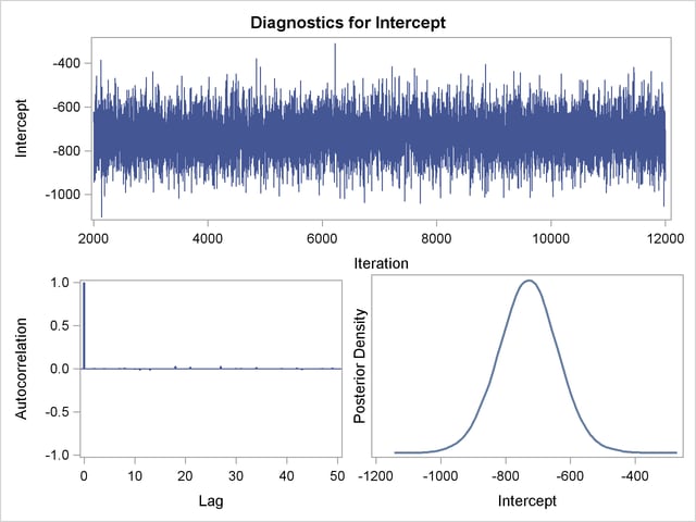
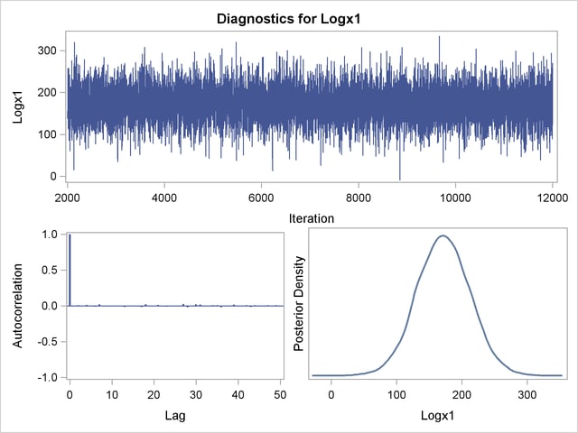
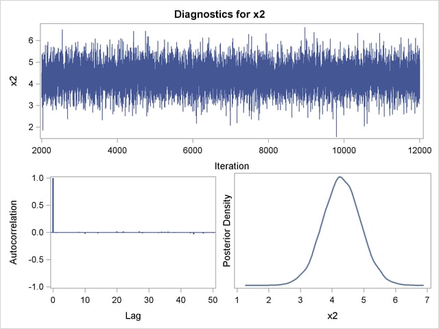
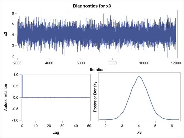
You should make sure that the posterior distribution samples have achieved convergence before using them for Bayesian inference. PROC GENMOD produces three convergence diagnostics by default. If ODS Graphics is enabled as specified in the following SAS statements, diagnostic plots are also displayed. See the section Assessing Markov Chain Convergence for more information about convergence diagnostics and their interpretation.
Summary statistics of the posterior distribution samples are produced by default. However, these statistics might not be sufficient for carrying out your Bayesian inference, and further processing of the posterior samples might be necessary. The following SAS statements request the Bayesian analysis, and the OUTPOST= option saves the samples in the SAS data set PostSurg for further processing:
ods graphics on;
proc genmod data=Surg;
   model y = Logx1 X2 X3 X4 / dist=normal;
   bayes seed=1 OutPost=PostSurg;
run;
ods graphics off;
The results of this analysis are shown in the following figures.
The "Model Information" table in Figure 37.8 summarizes information about the model you fit and the size of the simulation.
The "Analysis of Maximum Likelihood Parameter Estimates" table in Figure 37.9 summarizes maximum likelihood estimates of the model parameters.
| Analysis Of Maximum Likelihood Parameter Estimates | |||||
|---|---|---|---|---|---|
| Parameter | DF | Estimate | Standard Error | Wald 95% Confidence Limits | |
| Intercept | 1 | -730.559 | 85.4333 | -898.005 | -563.112 |
| Logx1 | 1 | 171.8758 | 38.2250 | 96.9561 | 246.7954 |
| x2 | 1 | 4.3019 | 0.5566 | 3.2109 | 5.3929 |
| x3 | 1 | 4.0309 | 0.4996 | 3.0517 | 5.0100 |
| x4 | 1 | 18.1377 | 12.0721 | -5.5232 | 41.7986 |
| Scale | 1 | 59.8591 | 5.7599 | 49.5705 | 72.2832 |
| Note: | The scale parameter was estimated by maximum likelihood. |
Since no prior distributions for the regression coefficients were specified, the default noninformative uniform distributions shown in the "Uniform Prior for Regression Coefficients" table in Figure 37.10 are used. Noninformative priors are appropriate if you have no prior knowledge of the likely range of values of the parameters, and if you want to make probability statements about the parameters or functions of the parameters. See, for example, Ibrahim, Chen, and Sinha (2001) for more information about choosing prior distributions.
The default noninformative gamma prior distribution for the normal scale parameter is shown in the "Independent Prior Distributions for Model Parameters" table in Figure 37.11.
By default, the maximum likelihood estimates of the regression parameters are used as the starting values for the simulation when noninformative prior distributions are used. These are listed in the "Initial Values and Seeds" table in Figure 37.12.
Summary statistics for the posterior sample are displayed in the "Fit Statistics," "Descriptive Statistics for the Posterior Sample," "Interval Statistics for the Posterior Sample," and "Posterior Correlation Matrix" tables in Figure 37.13, Figure 37.14, Figure 37.15, and Figure 37.16, respectively.
| Posterior Summaries | ||||||
|---|---|---|---|---|---|---|
| Parameter | N | Mean | Standard Deviation |
Percentiles | ||
| 25% | 50% | 75% | ||||
| Intercept | 10000 | -730.1 | 91.0133 | -789.6 | -729.6 | -670.5 |
| Logx1 | 10000 | 171.7 | 40.3792 | 144.3 | 171.8 | 198.6 |
| x2 | 10000 | 4.3000 | 0.5989 | 3.8990 | 4.2932 | 4.6951 |
| x3 | 10000 | 4.0310 | 0.5354 | 3.6645 | 4.0265 | 4.3910 |
| x4 | 10000 | 18.0888 | 12.8949 | 9.4919 | 18.0430 | 26.7881 |
| Dispersion | 10000 | 3795.9 | 770.4 | 3247.6 | 3694.7 | 4238.2 |
| Posterior Intervals | |||||
|---|---|---|---|---|---|
| Parameter | Alpha | Equal-Tail Interval | HPD Interval | ||
| Intercept | 0.050 | -908.7 | -551.0 | -906.2 | -549.2 |
| Logx1 | 0.050 | 92.4773 | 251.6 | 94.2813 | 253.0 |
| x2 | 0.050 | 3.1062 | 5.4839 | 3.1747 | 5.5328 |
| x3 | 0.050 | 2.9812 | 5.1041 | 2.9532 | 5.0612 |
| x4 | 0.050 | -7.2646 | 43.6506 | -5.9839 | 44.6427 |
| Dispersion | 0.050 | 2569.0 | 5548.5 | 2389.4 | 5308.8 |
| Posterior Correlation Matrix | ||||||
|---|---|---|---|---|---|---|
| Parameter | Intercept | Logx1 | x2 | x3 | x4 | Dispersion |
| Intercept | 1.000 | -0.856 | -0.580 | -0.712 | 0.579 | -0.002 |
| Logx1 | -0.856 | 1.000 | 0.285 | 0.490 | -0.636 | 0.009 |
| x2 | -0.580 | 0.285 | 1.000 | 0.302 | -0.492 | -0.007 |
| x3 | -0.712 | 0.490 | 0.302 | 1.000 | -0.616 | -0.004 |
| x4 | 0.579 | -0.636 | -0.492 | -0.616 | 1.000 | 0.002 |
| Dispersion | -0.002 | 0.009 | -0.007 | -0.004 | 0.002 | 1.000 |
Since noninformative prior distributions were used, the posterior sample means, standard deviations, and interval statistics shown in Figure 37.13 and Figure 37.14 are consistent with the maximum likelihood estimates shown in Figure 37.9.
By default, PROC GENMOD computes three convergence diagnostics: the lag1, lag5, lag10, and lag50 autocorrelations (Figure 37.17); Geweke diagnostic statistics (Figure 37.18); and effective sample sizes (Figure 37.19). There is no indication that the Markov chain has not converged. See the section Assessing Markov Chain Convergence for more information about convergence diagnostics and their interpretation.
| Posterior Autocorrelations | ||||
|---|---|---|---|---|
| Parameter | Lag 1 | Lag 5 | Lag 10 | Lag 50 |
| Intercept | -0.0050 | -0.0023 | -0.0138 | 0.0032 |
| Logx1 | 0.0030 | -0.0063 | -0.0070 | -0.0034 |
| x2 | -0.0113 | -0.0046 | -0.0235 | -0.0139 |
| x3 | 0.0019 | 0.0064 | -0.0073 | 0.0047 |
| x4 | -0.0001 | -0.0084 | 0.0050 | -0.0084 |
| Dispersion | -0.0019 | 0.0088 | -0.0297 | 0.0025 |
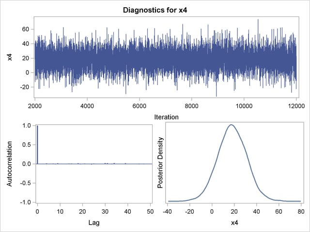
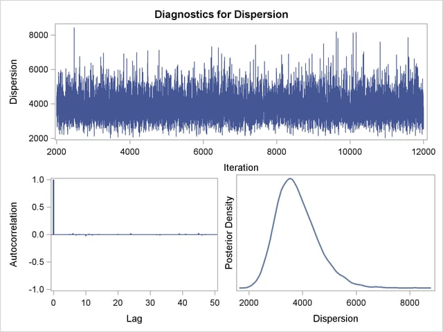
Trace, autocorrelation, and density plots for the seven model parameters, shown in Figure 37.20 through Figure 37.25, are useful in diagnosing whether the Markov chain of posterior samples has converged. These plots show no evidence that the chain has not converged. See the section Visual Analysis via Trace Plots for help with interpreting these diagnostic plots.
Suppose, for illustration, a question of scientific interest is whether blood clotting score has a positive effect on survival time. Since the model parameters are regarded as random quantities in a Bayesian analysis, you can answer this question by estimating the conditional probability of being positive, given the data, , from the posterior distribution samples. The following SAS statements compute the estimate of the probability of being positive:
data Prob;
   set PostSurg;
   Indicator = (logX1 > 0);
   label Indicator= 'log(Blood Clotting Score) > 0';
run;

proc Means data = Prob(keep=Indicator) n mean;
run;
As shown in Figure 37.26, there is a 1.00 probability of a positive relationship between the logarithm of a blood clotting score and survival time, adjusted for the other covariates.

Copyright © SAS Institute, Inc. All Rights Reserved.