| The FASTCLUS Procedure |
Getting Started: FASTCLUS Procedure
The following example demonstrates how to use the FASTCLUS procedure to compute disjoint clusters of observations in a SAS data set.
The data in this example are measurements taken on 159 freshwater fish caught from the same lake (Laengelmavesi) near Tampere in Finland. This data set is available from Puranen.
The species (bream, parkki, pike, perch, roach, smelt, and whitefish), weight, three different length measurements (measured from the nose of the fish to the beginning of its tail, the notch of its tail, and the end of its tail), height, and width of each fish are tallied. The height and width are recorded as percentages of the third length variable.
Suppose that you want to group empirically the fish measurements into clusters and that you want to associate the clusters with the species. You can use the FASTCLUS procedure to perform a cluster analysis.
The following DATA step creates the SAS data set Fish:
proc format;
   value specfmt
      1='Bream'
      2='Roach'
      3='Whitefish'
      4='Parkki'
      5='Perch'
      6='Pike'
      7='Smelt';
run;
data fish (drop=HtPct WidthPct);
   title 'Fish Measurement Data';
   input Species Weight Length1 Length2 Length3 HtPct WidthPct @@;

   *** transform variables;
   if Weight <= 0 or Weight =. then delete;
   Weight3=Weight**(1/3);
   Height=HtPct*Length3/(Weight3*100);
   Width=WidthPct*Length3/(Weight3*100);
   Length1=Length1/Weight3;
   Length2=Length2/Weight3;
   Length3=Length3/Weight3;
   logLengthRatio=log(Length3/Length1);

   format Species specfmt.;
   symbol = put(Species, specfmt2.);
   datalines;
1  242.0 23.2 25.4 30.0 38.4 13.4 1  290.0 24.0 26.3 31.2 40.0 13.8
1  340.0 23.9 26.5 31.1 39.8 15.1 1  363.0 26.3 29.0 33.5 38.0 13.3
1  430.0 26.5 29.0 34.0 36.6 15.1 1  450.0 26.8 29.7 34.7 39.2 14.2
1  500.0 26.8 29.7 34.5 41.1 15.3 1  390.0 27.6 30.0 35.0 36.2 13.4
1  450.0 27.6 30.0 35.1 39.9 13.8 1  500.0 28.5 30.7 36.2 39.3 13.7
1  475.0 28.4 31.0 36.2 39.4 14.1 1  500.0 28.7 31.0 36.2 39.7 13.3
1  500.0 29.1 31.5 36.4 37.8 12.0 1     .  29.5 32.0 37.3 37.3 13.6
1  600.0 29.4 32.0 37.2 40.2 13.9 1  600.0 29.4 32.0 37.2 41.5 15.0

   ... more lines ...

7   19.7 13.2 14.3 15.2 18.9 13.6 7   19.9 13.8 15.0 16.2 18.1 11.6
;
The double trailing at sign (@@) in the INPUT statement specifies that observations are input from each line until all values are read. The variables are rescaled in order to adjust for dimensionality. Because the new variables Weight3–logLengthRatio depend on the variable Weight, observations with missing values for Weight are not added to the data set. Consequently, there are 157 observations in the SAS data set Fish.
In the Fish data set, the variables are not measured in the same units and cannot be assumed to have equal variance. Therefore, it is necessary to standardize the variables before performing the cluster analysis.
The following statements standardize the variables and perform a cluster analysis on the standardized data:
proc standard data=Fish out=Stand mean=0 std=1;
   var Length1 logLengthRatio Height Width Weight3;
run;

proc fastclus data=Stand out=Clust
              maxclusters=7 maxiter=100 ;
   var Length1 logLengthRatio Height Width Weight3;
run;
The STANDARD procedure is first used to standardize all the analytical variables to a mean of 0 and standard deviation of 1. The procedure creates the output data set Stand to contain the transformed variables.
The FASTCLUS procedure then uses the data set Stand as input and creates the data set Clust. This output data set contains the original variables and two new variables, Cluster and Distance. The variable Cluster contains the cluster number to which each observation has been assigned. The variable Distance gives the distance from the observation to its cluster seed.
It is usually desirable to try several values of the MAXCLUSTERS= option. A reasonable beginning for this example is to use MAXCLUSTERS=7, since there are seven species of fish represented in the data set Fish.
The VAR statement specifies the variables used in the cluster analysis.
The results from this analysis are displayed in the following figures.
| Fish Measurement Data |
| Initial Seeds | |||||
|---|---|---|---|---|---|
| Cluster | Length1 | logLengthRatio | Height | Width | Weight3 |
| 1 | 1.388338414 | -0.979577858 | -1.594561848 | -2.254050655 | 2.103447062 |
| 2 | -1.117178039 | -0.877218192 | -0.336166276 | 2.528114070 | 1.170706464 |
| 3 | 2.393997461 | -0.662642015 | -0.930738701 | -2.073879107 | -1.839325419 |
| 4 | -0.495085516 | -0.964041012 | -0.265106856 | -0.028245072 | 1.536846394 |
| 5 | -0.728772773 | 0.540096664 | 1.130501398 | -1.207930053 | -1.107018207 |
| 6 | -0.506924177 | 0.748211648 | 1.762482687 | 0.211507596 | 1.368987826 |
| 7 | 1.573996573 | -0.796593995 | -0.824217424 | 1.561715851 | -1.607942726 |
Figure 34.1 displays the table of initial seeds used for each variable and cluster. The first line in the figure displays the option settings for REPLACE, RADIUS, MAXCLUSTERS, and MAXITER. These options, with the exception of MAXCLUSTERS and MAXITER, are set at their respective default values (REPLACE=FULL, RADIUS=0). Both the MAXCLUSTERS= and MAXITER= options are set in the PROC FASTCLUS statement.
Next, PROC FASTCLUS produces a table of summary statistics for the clusters. Figure 34.2 displays the number of observations in the cluster (frequency) and the root mean squared standard deviation. The next two columns display the largest Euclidean distance from the cluster seed to any observation within the cluster and the number of the nearest cluster.
The last column of the table displays the distance between the centroid of the nearest cluster and the centroid of the current cluster. A centroid is the point having coordinates that are the means of all the observations in the cluster.
| Cluster Summary | ||||||
|---|---|---|---|---|---|---|
| Cluster | Frequency | RMS Std Deviation | Maximum Distance from Seed to Observation |
Radius Exceeded |
Nearest Cluster | Distance Between Cluster Centroids |
| 1 | 17 | 0.5064 | 1.7781 | 4 | 2.5106 | |
| 2 | 19 | 0.3696 | 1.5007 | 4 | 1.5510 | |
| 3 | 13 | 0.3803 | 1.7135 | 1 | 2.6704 | |
| 4 | 13 | 0.4161 | 1.3976 | 7 | 1.4266 | |
| 5 | 11 | 0.2466 | 0.6966 | 6 | 1.7301 | |
| 6 | 34 | 0.3563 | 1.5443 | 5 | 1.7301 | |
| 7 | 50 | 0.4447 | 2.3915 | 4 | 1.4266 | |
Figure 34.3 displays the table of statistics for the variables. The table lists for each variable the total standard deviation, the pooled within-cluster standard deviation and the R-square value for predicting the variable from the cluster. The ratio of between-cluster variance to within-cluster variance ( to
to  ) appears in the last column.
| Statistics for Variables | ||||
|---|---|---|---|---|
| Variable | Total STD | Within STD | R-Square | RSQ/(1-RSQ) |
| Length1 | 1.00000 | 0.31428 | 0.905030 | 9.529606 |
| logLengthRatio | 1.00000 | 0.39276 | 0.851676 | 5.741989 |
| Height | 1.00000 | 0.20917 | 0.957929 | 22.769295 |
| Width | 1.00000 | 0.55558 | 0.703200 | 2.369270 |
| Weight3 | 1.00000 | 0.47251 | 0.785323 | 3.658162 |
| OVER-ALL | 1.00000 | 0.40712 | 0.840631 | 5.274764 |
The pseudo F statistic, approximate expected overall R square, and cubic clustering criterion (CCC) are listed at the bottom of the figure. You can compare values of these statistics by running PROC FASTCLUS with different values for the MAXCLUSTERS= option. The R square and CCC values are not valid for correlated variables.
Values of the cubic clustering criterion greater than 2 or 3 indicate good clusters. Values between 0 and 2 indicate potential clusters, but they should be taken with caution; large negative values can indicate outliers.
PROC FASTCLUS next produces the within-cluster means and standard deviations of the variables, displayed in Figure 34.4.
| Cluster Means | |||||
|---|---|---|---|---|---|
| Cluster | Length1 | logLengthRatio | Height | Width | Weight3 |
| 1 | 1.747808245 | -0.868605685 | -1.327226832 | -1.128760946 | 0.806373599 |
| 2 | -0.405231510 | -0.979113021 | -0.281064162 | 1.463094486 | 1.060450065 |
| 3 | 2.006796315 | -0.652725165 | -1.053213440 | -1.224020795 | -1.826752838 |
| 4 | -0.136820952 | -1.039312574 | -0.446429482 | 0.162596336 | 0.278560318 |
| 5 | -0.850130601 | 0.550190242 | 1.245156076 | -0.836585750 | -0.567022647 |
| 6 | -0.843912827 | 1.522291347 | 1.511408739 | -0.380323563 | 0.763114370 |
| 7 | -0.165570970 | -0.048881276 | -0.353723615 | 0.546442064 | -0.668780782 |
| Cluster Standard Deviations | |||||
|---|---|---|---|---|---|
| Cluster | Length1 | logLengthRatio | Height | Width | Weight3 |
| 1 | 0.3418476428 | 0.3544065543 | 0.1666302451 | 0.6172880027 | 0.7944227150 |
| 2 | 0.3129902863 | 0.3592350778 | 0.1369052680 | 0.5467406493 | 0.3720119097 |
| 3 | 0.2962504486 | 0.1740941675 | 0.1736086707 | 0.7528475622 | 0.0905232968 |
| 4 | 0.3254364840 | 0.2836681149 | 0.1884592934 | 0.4543390702 | 0.6612055341 |
| 5 | 0.1781837609 | 0.0745984121 | 0.2056932592 | 0.2784540794 | 0.3832002850 |
| 6 | 0.2273744242 | 0.3385584051 | 0.2046010964 | 0.5143496067 | 0.4025849044 |
| 7 | 0.3734733622 | 0.5275768119 | 0.2551130680 | 0.5721303628 | 0.4223181710 |
It is useful to study further the clusters calculated by the FASTCLUS procedure. One method is to look at a frequency tabulation of the clusters with other classification variables. The following statements invoke the FREQ procedure to crosstabulate the empirical clusters with the variable Species:
proc freq data=Clust;
   tables Species*Cluster;
run;
Figure 34.5 displays the marked division between clusters.
| Fish Measurement Data |
|
|
|||||||||||||||||||||||||||||||||||||||||||||||||||||||||||||||||||||||||||||||||||||||||||||||||||||||||||||||||||||||||||||||||||||||||||||||||||||||||||||||||||||||||||||||||||||||||||||||||||||||||||||||||||||||||||||||||||||||||||||||||||||||||||||||||||||||||||||||||||||||||||||||||||||||||||||||||||||||||||||||||||||||||||||||||||
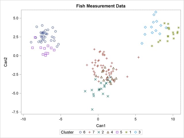
For cases in which you have three or more clusters, you can use the CANDISC and SGPLOT procedures to obtain a graphical check on the distribution of the clusters. In the following statements, the CANDISC and SGPLOT procedures are used to compute canonical variables and plot the clusters:
proc candisc data=Clust out=Can noprint;
   class Cluster;
   var Length1 logLengthRatio Height Width Weight3;
run;

proc sgplot data=Can;
   scatter y=Can2 x=Can1 / group=Cluster ;
run;
First, the CANDISC procedure is invoked to perform a canonical discriminant analysis by using the data set Clust and creating the output SAS data set Can. The NOPRINT option suppresses display of the output. The CLASS statement specifies the variable Cluster to define groups for the analysis. The VAR statement specifies the variables used in the analysis.
Next, the SGPLOT procedure plots the two canonical variables from PROC CANDISC, Can1 and Can2. The PLOT statement specifies the variable Cluster as the identification variable. The resulting plot (Figure 34.6) illustrates the spatial separation of the clusters calculated in the FASTCLUS procedure.
Copyright © SAS Institute, Inc. All Rights Reserved.