Let be a spatial random field (SRF) with measured values at respective locations , . You use the VARIOGRAM procedure because you want to gain insight into the spatial continuity and structure of . A good measure of the spatial continuity of is defined by means of the variance of the difference , where and are locations in . Specifically, if you consider and to be spatial increments such that , then the variance function based on the increments is independent of the actual locations , . Most commonly, the continuity measure used in practice is one half of this variance, better known as the semivariance function:

or, equivalently,

The plot of semivariance as a function of is the semivariogram. In extension to its meaning, you might commonly see the term semivariogram used instead of the term semivariance, as well.

Assume that the SRF is free of nonrandom (or systematic) surface trends. Then, the expected value of will be a constant for all , and the semivariance expression is simplified to the following:

Given the preceding assumption, you can compute an estimate of the semivariance from a finite set of points in a practical way by using the formula

where the sets contain all the neighboring pairs at distance :

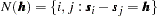and is the number of such pairs .

The expression for is called the empirical semivariance (Matheron; 1963). This is the quantity that PROC VARIOGRAM computes, and its corresponding plot is the empirical semivariogram. According to Cressie (1993, p. 96), the estimate has approximate variance

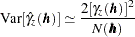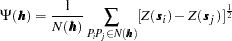
The empirical semivariance is also referred to as classical. This name is used so that it can be distinguished from the robust semivariance estimate and the corresponding robust semivariogram. The robust semivariance was introduced by Cressie and Hawkins (1980) and is described by Cressie (1993, p. 75) as:

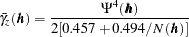In the preceding expression the parameter is defined as:

Note that if your data include a surface trend, then the empirical semivariance is not an estimate of the theoretical semivariance function . Instead, rather than the spatial increments variance, it represents a different quantity known as pseudo-semivariance, and its corresponding plot is a pseudo-semivariogram. In principle, pseudo-semivariograms do not provide measures of the spatial continuity. They can thus lead to misinterpretations of the spatial structure, and are consequently unsuitable for the purpose of spatial prediction. For further information, see the detailed discussion in the section Empirical Semivariograms and Surface Trends. Under certain conditions you might be able to gain some insight about the spatial continuity with a pseudo-semivariogram. This case is presented in Analysis without Surface Trend Removal.