The TREE Procedure

Getting Started: TREE Procedure

The TREE procedure creates tree diagrams from a SAS data set containing the tree structure. You can create this type of data set with the CLUSTER or VARCLUS procedure. See Chapter 29, The CLUSTER Procedure, and Chapter 93, The VARCLUS Procedure, for more information.

In the following example, the VARCLUS procedure is used to divide a set of variables into hierarchical clusters and to create the SAS data set containing the tree structure. The TREE procedure then generates the tree diagrams.

The following data, from Hand et al. (1994), represent the amount of protein consumed from nine food groups for each of 25 European countries. The nine food groups are red meat (RedMeat), white meat (WhiteMeat), eggs (Eggs), milk (Milk), fish (Fish), cereal (Cereal), starch (Starch), nuts (Nuts), and fruits and vegetables (FruVeg).

The following SAS statements create the data set Protein:

   data Protein;                                                        
      input Country $15. RedMeat WhiteMeat Eggs Milk
         Fish Cereal Starch Nuts FruVeg;
      datalines;
   Albania        10.1  1.4  0.5   8.9  0.2  42.3  0.6  5.5  1.7
   Austria         8.9 14.0  4.3  19.9  2.1  28.0  3.6  1.3  4.3   
   Belgium        13.5  9.3  4.1  17.5  4.5  26.6  5.7  2.1  4.0
   Bulgaria        7.8  6.0  1.6   8.3  1.2  56.7  1.1  3.7  4.2
   Czechoslovakia  9.7 11.4  2.8  12.5  2.0  34.3  5.0  1.1  4.0
   Denmark        10.6 10.8  3.7  25.0  9.9  21.9  4.8  0.7  2.4
   E Germany       8.4 11.6  3.7  11.1  5.4  24.6  6.5  0.8  3.6
   Finland         9.5  4.9  2.7  33.7  5.8  26.3  5.1  1.0  1.4
   France         18.0  9.9  3.3  19.5  5.7  28.1  4.8  2.4  6.5
   Greece         10.2  3.0  2.8  17.6  5.9  41.7  2.2  7.8  6.5
   Hungary         5.3 12.4  2.9   9.7  0.3  40.1  4.0  5.4  4.2
   Ireland        13.9 10.0  4.7  25.8  2.2  24.0  6.2  1.6  2.9
   Italy           9.0  5.1  2.9  13.7  3.4  36.8  2.1  4.3  6.7
   Netherlands     9.5 13.6  3.6  23.4  2.5  22.4  4.2  1.8  3.7
   Norway          9.4  4.7  2.7  23.3  9.7  23.0  4.6  1.6  2.7
   Poland          6.9 10.2  2.7  19.3  3.0  36.1  5.9  2.0  6.6
   Portugal        6.2  3.7  1.1   4.9 14.2  27.0  5.9  4.7  7.9
   Romania         6.2  6.3  1.5  11.1  1.0  49.6  3.1  5.3  2.8
   Spain           7.1  3.4  3.1   8.6  7.0  29.2  5.7  5.9  7.2
   Sweden          9.9  7.8  3.5   4.7  7.5  19.5  3.7  1.4  2.0
   Switzerland    13.1 10.1  3.1  23.8  2.3  25.6  2.8  2.4  4.9
   UK             17.4  5.7  4.7  20.6  4.3  24.3  4.7  3.4  3.3
   USSR            9.3  4.6  2.1  16.6  3.0  43.6  6.4  3.4  2.9
   W Germany      11.4 12.5  4.1  18.8  3.4  18.6  5.2  1.5  3.8
   Yugoslavia      4.4  5.0  1.2   9.5  0.6  55.9  3.0  5.7  3.2
   ;                                                            
   run;

The data set Protein contains the character variable Country and the nine numeric variables representing the food groups. The $15. in the INPUT statement specifies that the variable Country is a character variable with a length of 15.

The following statements cluster the variables in the data set Protein. The OUTTREE= option creates an output data set named Tree to contain the tree structure. The CENTROID option specifies the centroid clustering method, and the MAXCLUSTERS= option specifies that the largest number of clusters desired is four. The NOPRINT option suppresses the display of the output. The VAR statement specifies that all numeric variables (RedMeat—FruVeg) are used by the procedure.

   proc varclus data=Protein outtree=Tree centroid maxclusters=4 noprint;
      var RedMeat--FruVeg;
   run;

The output data set Tree, created by the OUTTREE= option in the previous statements, contains the following variables:

_NAME_: the name of the cluster
_PARENT_: the parent of the cluster
_NCL_: the number of clusters
_VAREXP_: the amount of variance explained by the cluster
_PROPOR_: the proportion of variance explained by the clusters at the current level of the tree diagram
_MINPRO_: the minimum proportion of variance explained by a cluster
_MAXEIGEN_: the maximum second eigenvalue of a cluster

The following statements produce tree diagrams of the clusters created by PROC VARCLUS:

   proc tree data=tree;

   proc tree data=tree lineprinter;

PROC TREE is invoked twice. In the first invocation, the tree diagram is presented using the default graphical output. In the second invocation, the LINEPRINTER option specifies line printer output.

Figure 91.1 displays the default graphical representation of the tree diagram.

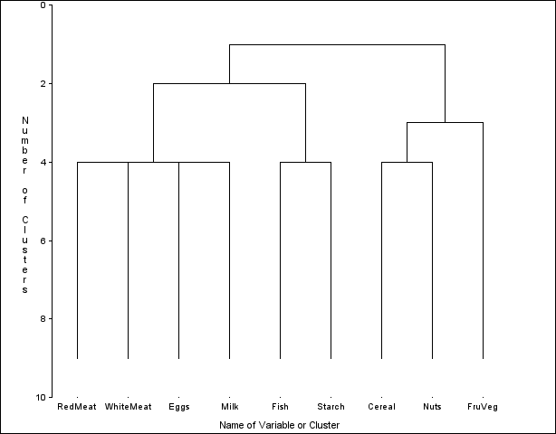
Figure 91.1 Graphical Tree Diagram from PROC TREE

Figure 91.2 displays the same information as Figure 91.1 by using line printer output.

Figure 91.2 Line Printer Representation of the Tree Diagram

The TREE Procedure

Oblique Centroid Component Clustering

                             Name of Variable or Cluster                        
                                                                                
                        W                                                       
                        h                                                       
                  R     i                                                       
                  e     t                       S     C           F             
                  d     e                       t     e           r             
                  M     M     E     M     F     a     r     N     u             
                  e     e     g     i     i     r     e     u     V             
                  a     a     g     l     s     c     a     t     e             
                  t     t     s     k     h     h     l     s     g             
               1 +XXXXXXXXXXXXXXXXXXXXXXXXXXXXXXXXXXXXXXXXXXXXXXXXX             
                 |XXXXXXXXXXXXXXXXXXXXXXXXXXXXXXX     XXXXXXXXXXXXX             
                 |XXXXXXXXXXXXXXXXXXXXXXXXXXXXXXX     XXXXXXXXXXXXX             
            N  2 +XXXXXXXXXXXXXXXXXXXXXXXXXXXXXXX     XXXXXXXXXXXXX             
            u    |XXXXXXXXXXXXXXXXXXX     XXXXXXX     XXXXXXXXXXXXX             
            m    |XXXXXXXXXXXXXXXXXXX     XXXXXXX     XXXXXXXXXXXXX             
            b  3 +XXXXXXXXXXXXXXXXXXX     XXXXXXX     XXXXXXXXXXXXX             
            e    |XXXXXXXXXXXXXXXXXXX     XXXXXXX     XXXXXXX     .             
            r    |XXXXXXXXXXXXXXXXXXX     XXXXXXX     XXXXXXX     .             
               4 +XXXXXXXXXXXXXXXXXXX     XXXXXXX     XXXXXXX     .             
            o    |.     .     .     .     .     .     .     .     .             
            f    |.     .     .     .     .     .     .     .     .             
               5 +.     .     .     .     .     .     .     .     .             
            C    |.     .     .     .     .     .     .     .     .             
            l    |.     .     .     .     .     .     .     .     .             
            u  6 +.     .     .     .     .     .     .     .     .             
            s    |.     .     .     .     .     .     .     .     .             
            t    |.     .     .     .     .     .     .     .     .             
            e  7 +.     .     .     .     .     .     .     .     .             
            r    |.     .     .     .     .     .     .     .     .             
            s    |.     .     .     .     .     .     .     .     .             
               8 +.     .     .     .     .     .     .     .     .             
                 |.     .     .     .     .     .     .     .     .             
                 |.     .     .     .     .     .     .     .     .             
               9 +.     .     .     .     .     .     .     .     .

In each diagram the name of the cluster is displayed on the horizontal axis and the number of clusters is displayed on the vertical or height axis.

As you look up from the bottom of either diagram, clusters are progressively joined until a single, all-encompassing cluster is formed at the top (or root) of the tree. Clusters exist at each level of the diagram. For example, at the level where the diagram indicates three clusters, the clusters are as follows:

Cluster 1: RedMeat WhiteMeat Eggs Milk
Cluster 2: Fish Starch
Cluster 3: Cereal Nuts FruVeg

As you proceed up the diagram one level, the number of clusters is two:

Cluster 1: RedMeat WhiteMeat Eggs Milk Fish Starch
Cluster 2: Cereal Nuts FruVeg

The following statements illustrate how you can specify the numeric variable defining the height of each node (cluster) in the tree:

   axis1 order=(0 to 1 by 0.2);
   proc tree data=Tree horizontal haxis=axis1;
      height _PROPOR_;
   run;

The AXIS1 statement ORDER= option specifies the data values in the order in which they are to appear on the axis. The HORIZONTAL option in the PROC TREE statement orients the tree diagram horizontally. The HAXIS option specifies that the AXIS1 statement be used to customize the appearance of the horizontal axis. The HEIGHT statement specifies the variable _PROPOR_ (the proportion of variance explained) as the height variable.

The resulting tree diagram is shown in Figure 91.3.

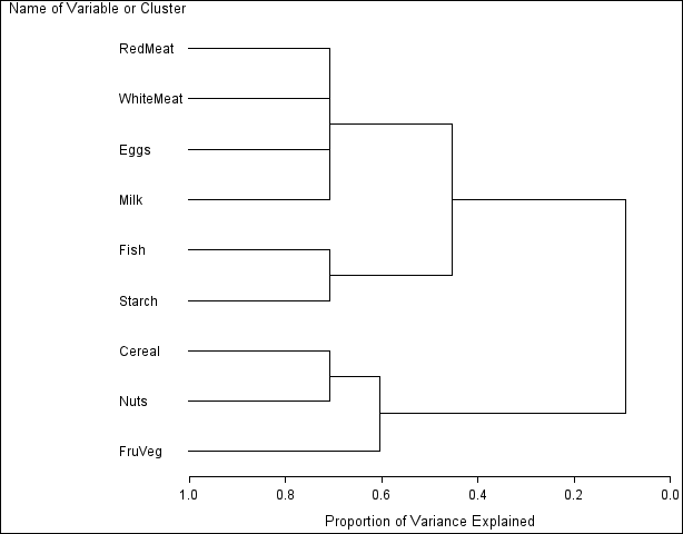
Figure 91.3 Horizontal Tree Diagram with _PROPOR_ as the HEIGHT Variable

As you look from left to right in the diagram, objects and clusters are progressively joined until a single, all-encompassing cluster is formed at the right (or root) of the tree.

Clusters exist at each level of the diagram, represented by horizontal line segments. Each vertical line segment represents a point where leaves and branches are connected into progressively larger clusters.

For example, three clusters are formed at the leftmost point along the axis where three horizontal line segments exist. At that point, where a vertical line segment connects the Cereal-Nuts and FruVeg clusters, the proportion of variance explained is about 0.6 (_PROPOR_ = 0.6). At the next clustering level the variables Fish and Starch are clustered with variables RedMeat through Milk, resulting in a total of two clusters. The proportion of variance explained is about 0.45 at that point.

Top of Page