| The TPSPLINE Procedure |
Example 89.3 Multiple Minima of the GCV Function
The data in this example represent the deposition of sulfate (SO ) at
) at  sites in the
  contiguous states of the United States in 1990. Each observation records the latitude and longitude of the site as well as the SO deposition at the site measured in grams per square meter (
 ).
).
You can use PROC TPSPLINE to fit a surface that reflects the general trend and that reveals underlying features of the data, which are shown in the following DATA step:
   data so4;
   input latitude longitude so4 @@;
   datalines;
   32.45833  87.24222 1.403 34.28778  85.96889 2.103
   33.07139 109.86472 0.299 36.07167 112.15500 0.304
   31.95056 112.80000 0.263 33.60500  92.09722 1.950

   ... more lines ...

   43.87333 104.19222 0.306 44.91722 110.42028 0.210
   45.07611  72.67556 2.646
   ;
   data pred;
      do latitude = 25 to 47 by 1;
         do longitude = 68 to 124 by 1;
            output;
         end;
      end;
   run;
The preceding statements create the SAS data set so4 and the data set pred in order to make predictions on a regular grid. The following statements fit a surface for SO deposition. The ODS OUTPUT statement creates a data set called GCV to contain the GCV values for LOGNLAMBDA in the range from  to
to  .
.
   proc tpspline data=so4;
      ods output GCVFunction=gcv;
      model so4 = (latitude longitude) /lognlambda=(-6 to 1 by 0.1);
      score data=pred out=prediction1;
   run;
Partial output from these statements is displayed in Output 89.3.1 and Output 89.3.2.

| Summary of Input Data Set | |
|---|---|
| Number of Non-Missing Observations | 179 |
| Number of Missing Observations | 0 |
| Unique Smoothing Design Points | 179 |
The following statements use PROC TEMPLATE to produce Output 89.3.3:
   proc template;
   define statgraph plotgcv;
   begingraph;
      entrytitle "GCV Function";
      layout overlay/xaxisopts=(griddisplay=on label="log_10 (n * Lambda)")
                     yaxisopts=(griddisplay=on label="GCV values");
                     seriesplot x=lognlambda y=gcv;
      endlayout;
   endgraph;
   end;
   run;

   ods graphics on;

   proc sgrender data=gcv template=plotgcv;run;
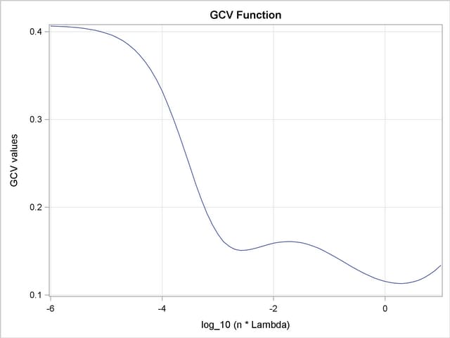
Output 89.3.3 displays the plot of the GCV function versus NLAMBDA in  scale. The GCV function has two minima. PROC TPSPLINE locates the global minimum at
  . The plot also displays a local minimum located around
  . Note that the TPSPLINE procedure might not always find the global minimum, although it did in this case.
Data Set
The following analysis specifies the option LOGNLAMBDA0=. The output is displayed in Output 89.3.4.
   proc tpspline data=so4;
      model so4 = (latitude longitude) /lognlambda0=-2.56;
      score data=pred out=prediction2;
   run;
with LOGNLAMBDA=
| Summary of Input Data Set | |
|---|---|
| Number of Non-Missing Observations | 179 |
| Number of Missing Observations | 0 |
| Unique Smoothing Design Points | 179 |
| Summary of Final Model | |
|---|---|
| Number of Regression Variables | 0 |
| Number of Smoothing Variables | 2 |
| Order of Derivative in the Penalty | 2 |
| Dimension of Polynomial Space | 3 |
| Summary Statistics of Final Estimation | |
|---|---|
| log10(n*Lambda) | -2.5600 |
| Smoothing Penalty | 177.2144 |
| Residual SS | 0.0438 |
| Tr(I-A) | 7.2086 |
| Model DF | 171.7914 |
| Standard Deviation | 0.0779 |
The smoothing penalty in Output 89.3.4 is much larger than that displayed in Output 89.3.1. The estimate in Output 89.3.1 uses a large  value and, therefore, the surface is smoother than the estimate by using LOGNLAMBDA= (Output 89.3.4).
The estimate based on LOGNLAMBDA= has a larger value for the degrees of freedom, and it has a much smaller standard deviation.
However, a smaller standard deviation in nonparametric regression does not necessarily mean that the estimate is good: a small value always produces an estimate closer to the data and, therefore, a smaller standard deviation.
The following statements use PROC TEMPLATE to define a template to produce two contour plots of the estimates by the two minima. A graph of two contour plots is then rendered by the SGRENDER procedure.
   proc template;
   define statgraph two_contour;
   begingraph /designheight=360;
      entrytitle "TPSPLINE Fits";
      layout lattice / columns=2 rows=1
                       columndatarange=unionall
                       rowdatarange=unionall
                       columngutter=10;
         rowaxes;
            rowaxis / offsetmin=0 offsetmax=0 display=all
                      linearopts=(thresholdmin=0 thresholdmax=0);
         endrowaxes;

         layout overlay/
            xaxisopts=(offsetmin=0 offsetmax=0
                       linearopts=(thresholdmin=0 thresholdmax=0))
            yaxisopts=(display=none);
            entry "lognlambda = 0.277"/location=outside valign=top
                  textattrs=graphlabeltext;
            scatterplot x=longitude y=latitude /primary=true markerattrs=(size=0);
            contourplotparm x=longitude y=latitude z=P_so4/
                          name="cont1" nlevels=5
                          contourtype=gradient;
            contourplotparm x=longitude y=latitude z=P_so4/
                          contourtype=labeledline nlevels=5;
         endlayout;

         layout overlay/
            xaxisopts=(offsetmin=0 offsetmax=0
                       linearopts=(thresholdmin=0 thresholdmax=0))
            yaxisopts=(display=none);
            entry "loglambda = -2.56"/location=outside valign=top
                  textattrs=graphlabeltext;
            scatterplot x=longitude y=latitude /primary=true markerattrs=(size=0);
            contourplotparm x=longitude y=latitude z=P_so4_b/
                          name="cont2" nlevels=5
                          contourtype=gradient;
            contourplotparm x=longitude y=latitude z=P_so4_b/
                          contourtype=labeledline nlevels=5;
         endlayout;

         row2headers;
            continuouslegend "cont1" / title="Predicted SO4" pad=(left=10);
         endrow2headers;

      endlayout;
   endgraph;
   end;
   run;
Compare the two estimates by examining the contour plots of both estimates (Output 89.3.5).
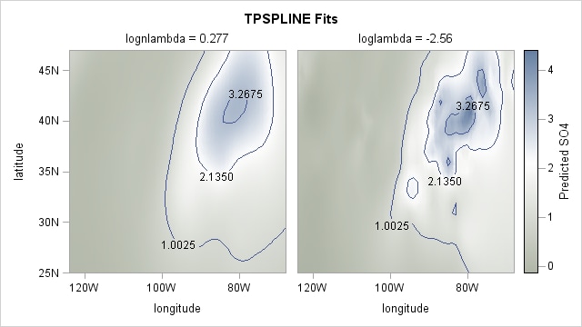
As the contour plots show, the estimate with LOGNLAMBDA=0.277 might represent the underlying trend, while the estimate with the LOGNLAMBDA=–2.56 is very rough and might be modeling the noise component.
Copyright © 2009 by SAS Institute Inc., Cary, NC, USA. All rights reserved.