| The SEQTEST Procedure |
Example 78.8 Testing an Effect in a Logistic Regression Model
This example requests a two-sided test for the dose effect in a dose-response model (Whitehead 1997, pp. 262–263). Consider the logistic regression model
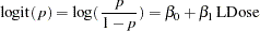 |
where  is the response probability to be modeled for the binary response Resp and LDose = log( Dose +1) is the covariate. The dose levels are
  for the control group, and they are
  ,
,  , and
, and  for the three treatment groups.
Following the derivations in the section "Test for a Parameter in the Logistic Regression Model" in the chapter "The SEQDESIGN Procedure," the required sample size can be derived from
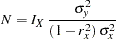 |
where  is the variance of the response variable in the logistic regression model,
  is the proportion of variance of LDose explained by other covariates, and
  is the variance of LDose.
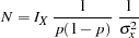
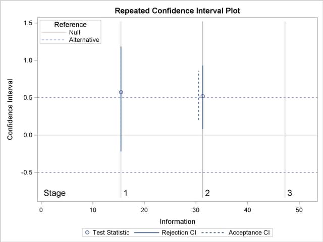
Since LDose is the only covariate in the model,  . For a logistic model, the variance
  can be estimated by
 |
where  is the estimated probability of the response variable Resp. Thus, the sample size can be computed as
 |
The null hypothesis  corresponds to no treatment effect. Suppose that the alternative hypothesis
  is the reference improvement that should be detected at a
  level.
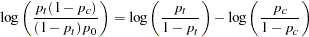
Note that  corresponds to an odds ratio of
  between the treatment group with dose level and the control group. The log odds ratio between the two groups is
 |
which corresponds to
 |
If the same number of patients are assigned in each of the four groups, then the MLE of the variance of LDose is  . Further, if the response rate is
  , then the required sample size can be derived using the SAMPLESIZE statement in the SEQDESIGN procedure.
The following statements invoke the SEQDESIGN procedure and request a three-stage group sequential design for normally distributed data. The design has a null hypothesis of no treatment effect with early stopping to reject the null hypothesis with a two-sided alternative hypothesis  .
.
   ods graphics on;
   proc seqdesign altref=0.5;
      TwoSidedErrorSpending: design method=errfuncpow
                                    method(loweralpha)=errfuncpow(rho=1)
                                    method(upperalpha)=errfuncpow(rho=3)
                                    nstages=3
                                    stop=both;
      samplesize model=logistic( prop=0.4 xvariance=0.5345);
   ods output Boundary=Bnd_Dose;
   run;
   ods graphics off;
The ODS OUTPUT statement with the BOUNDARY=BND_DOSE option creates an output data set named BND_DOSE which contains the resulting boundary information for the subsequent sequential tests.
The "Design Information" table in Output 78.8.1 displays design specifications and derived statistics. Since the alternative reference is specified, the maximum information  is derived.
| Design Information | |
|---|---|
| Statistic Distribution | Normal |
| Boundary Scale | Standardized Z |
| Alternative Hypothesis | Two-Sided |
| Early Stop | Accept/Reject Null |
| Method | Error Spending |
| Boundary Key | Both |
| Alternative Reference | 0.5 |
| Number of Stages | 3 |
| Alpha | 0.05 |
| Beta (Lower) | 0.1 |
| Beta (Upper) | 0.07871 |
| Power (Lower) | 0.9 |
| Power (Upper) | 0.92129 |
| Max Information (Percent of Fixed Sample) | 103.7223 |
| Max Information | 47.22445 |
| Null Ref ASN (Percent of Fixed Sample) | 79.47628 |
| Lower Alt Ref ASN (Sample Size) | 234.1646 |
| Upper Alt Ref ASN (Sample Size) | 270.4058 |
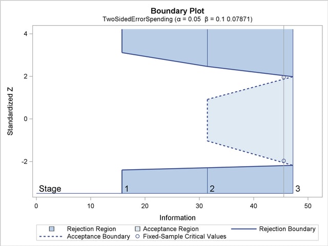
The "Boundary Information" table in Output 78.8.2 displays the information level, alternative reference, and boundary values at each stage. With the default BOUNDARYSCALE=STDZ option, the boundary values are displayed with the standardized  statistic scale.
| Boundary Information (Standardized Z Scale) Null Reference = 0 |
|||||||||
|---|---|---|---|---|---|---|---|---|---|
| _Stage_ | Alternative | Boundary Values | |||||||
| Information Level | Reference | Lower | Upper | ||||||
| Proportion | Actual | N | Lower | Upper | Alpha | Beta | Beta | Alpha | |
| 1 | 0.3333 | 15.74148 | 122.7119 | -1.98378 | 1.98378 | -2.39398 | . | . | 3.11302 |
| 2 | 0.6667 | 31.48297 | 245.4238 | -2.80548 | 2.80548 | -2.29380 | -1.02812 | 0.91855 | 2.46193 |
| 3 | 1.0000 | 47.22445 | 368.1357 | -3.43600 | 3.43600 | -2.17479 | -2.17479 | 1.98311 | 1.98311 |
With the specified ODS GRAPHICS ON statement, a detailed boundary plot with the rejection and acceptance regions is displayed by default, as shown in Output 78.8.3.
With the SAMPLESIZE statement, the "Sample Size Summary" table in Output 78.8.4 displays the parameters for the sample size computation.
The "Sample Sizes" table in Output 78.8.5 displays the required sample sizes for the group sequential clinical trial.
That is,  new patients are needed in each stage and the number is rounded up to
  for each stage to have a multiple of four for the four dose levels in the trial. Note that since the sample sizes are derived from an estimated response probability and are rounded up, the actual information levels might not match the corresponding target information levels.
Output 78.8.6 lists the first  observations of the trial data.
The following statements use the LOGISTIC procedure to estimate the slope  and its associated standard error at stage :
   proc logistic data=Dose_1;
      model Resp(event='1')= LDose;
      ods output ParameterEstimates=Parms_Dose1;
   run;
The following statements create and display (in Output 78.8.7) the input data set that contains slope  and its associated standard error for the SEQTEST procedure:
   data Parms_Dose1;
      set Parms_Dose1;
      if Variable='LDose';
      _Scale_='MLE';
      _Stage_= 1;
      keep _Scale_ _Stage_ Variable Estimate StdErr;
   run;

   proc print data=Parms_Dose1;
      title 'Statistics Computed at Stage 1';
   run;
The following statements invoke the SEQTEST procedure to test for early stopping at stage :
   ods graphics on;
   proc seqtest Boundary=Bnd_Dose
                Parms(testvar=LDose)=Parms_Dose1
                order=mle
                boundaryscale=mle
                ;
   ods output Test=Test_Dose1;
   run;
   ods graphics off;
The BOUNDARY= option specifies the input data set that provides the boundary information for the trial at stage , which was generated in the SEQDESIGN procedure. The PARMS=PARMS_DOSE1 option specifies the input data set PARMS_DOSE1 that contains the test statistic and its associated standard error at stage , and the TESTVAR=LDOSE option identifies the test variable LDOSE in the data set.
The ORDER=MLE option uses the MLE ordering to derive the  -value, the unbiased median estimate, and the confidence limits for the regression slope estimate.
The ODS OUTPUT statement with the TEST=TEST_DOSE1 option creates an output data set named TEST_DOSE1 which contains the updated boundary information for the test at stage . The data set also provides the boundary information that is needed for the group sequential test at the next stage.
The "Design Information" table in Output 78.8.8 displays design specifications. By default, the boundary values are modified for the new information levels to maintain the Type I  level. The maximum information remains the same as the design stored in the BOUNDARY= data set, but the derived Type II error probability
  and power
  are different because of the new information levels.
| Design Information | |
|---|---|
| BOUNDARY Data Set | WORK.BND_DOSE |
| Data Set | WORK.PARMS_DOSE1 |
| Statistic Distribution | Normal |
| Boundary Scale | MLE |
| Alternative Hypothesis | Two-Sided |
| Early Stop | Accept/Reject Null |
| Number of Stages | 3 |
| Alpha | 0.05 |
| Beta (Lower) | 0.09992 |
| Beta (Upper) | 0.07871 |
| Power (Lower) | 0.90008 |
| Power (Upper) | 0.92129 |
| Max Information (Percent of Fixed Sample) | 103.7231 |
| Max Information | 47.2244524 |
| Null Ref ASN (Percent of Fixed Sample) | 79.45049 |
| Lower Alt Ref ASN (Percent of Fixed Sample) | 66.05269 |
| Upper Alt Ref ASN (Percent of Fixed Sample) | 76.24189 |
The "Test Information" table in Output 78.8.9 displays the boundary values for the test statistic with the specified MLE scale.
| Test Information (MLE Scale) Null Reference = 0 |
||||||||||
|---|---|---|---|---|---|---|---|---|---|---|
| _Stage_ | Alternative | Boundary Values | Test | |||||||
| Information Level | Reference | Lower | Upper | LDose | ||||||
| Proportion | Actual | Lower | Upper | Alpha | Beta | Beta | Alpha | Estimate | Action | |
| 1 | 0.3272 | 15.45062 | -0.50000 | 0.50000 | -0.61078 | . | . | 0.79337 | 0.57409 | Continue |
| 2 | 0.6636 | 31.33753 | -0.50000 | 0.50000 | -0.40974 | -0.18169 | 0.16222 | 0.44033 | . | |
| 3 | 1.0000 | 47.22445 | -0.50000 | 0.50000 | -0.31633 | -0.31633 | 0.28860 | 0.28860 | . | |
The information level at stage is derived from the standard error  in the PARMS= data set,
 |
The remaining interim information levels are derived proportionally from the corresponding information levels in the original design. At stage , the boundary values are missing and there is no early stopping to accept  . The MLE statistic
  is between the lower and upper boundaries, so the trial continues to the next stage.
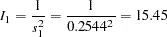
With the specified ODS GRAPHICS ON statement, a boundary plot with the boundary values and test statistics is displayed, as shown in Output 78.8.10. As expected, the test statistic is in the continuation region below the upper alpha boundary.

The following statements use the LOGISTIC procedure to estimate the slope and its associated standard error at stage :
   proc logistic data=dose_2;
      model Resp(event='1')=LDose;
      ods output ParameterEstimates=Parms_Dose2;
   run;
The following statements create and display (in Output 78.8.11) the input data set that contains slope and its associated standard error at stage for the SEQTEST procedure:
   data Parms_Dose2;
      set Parms_Dose2;
      if Variable='LDose';
      _Scale_='MLE';
      _Stage_= 2;
      keep _Scale_ _Stage_ Variable Estimate StdErr;
   run;

   proc print data=Parms_Dose2;
      title 'Statistics Computed at Stage 2';
   run;
The following statements invoke the SEQTEST procedure to test for early stopping at stage :
   ods graphics on;
   proc seqtest Boundary=Test_Dose1
                Parms(Testvar=LDose)=Parms_Dose2
                order=mle
                boundaryscale=mle
                rci
                plots=rci
                ;
   ods output Test=Test_Dose2;
   run;
   ods graphics off;
The BOUNDARY= option specifies the input data set that provides the boundary information for the trial at stage , which was generated by the SEQTEST procedure at the previous stage. The PARMS= option specifies the input data set that contains the test statistic and its associated standard error at stage , and the TESTVAR= option identifies the test variable in the data set.
The ORDER=MLE option uses the MLE ordering to derive the -value, unbiased median estimate, and confidence limits for the regression slope estimate.
The ODS OUTPUT statement with the TEST=TEST_DOSE2 option creates an output data set named TEST_DOSE2 which contains the updated boundary information for the test at stage . The data set also provides the boundary information that is needed for the group sequential test at the next stage.
The "Design Information" table in Output 78.8.12 displays design specifications. By default, the boundary values are modified for the new information levels to maintain the Type I level.
| Design Information | |
|---|---|
| BOUNDARY Data Set | WORK.TEST_DOSE1 |
| Data Set | WORK.PARMS_DOSE2 |
| Statistic Distribution | Normal |
| Boundary Scale | MLE |
| Alternative Hypothesis | Two-Sided |
| Early Stop | Accept/Reject Null |
| Number of Stages | 3 |
| Alpha | 0.05 |
| Beta (Lower) | 0.0999 |
| Beta (Upper) | 0.07871 |
| Power (Lower) | 0.9001 |
| Power (Upper) | 0.92129 |
| Max Information (Percent of Fixed Sample) | 103.7227 |
| Max Information | 47.2244524 |
| Null Ref ASN (Percent of Fixed Sample) | 79.44086 |
| Lower Alt Ref ASN (Percent of Fixed Sample) | 66.04641 |
| Upper Alt Ref ASN (Percent of Fixed Sample) | 76.22739 |
The information is derived from the standard error associated with the slope estimate at the final stage and is larger than the target level. The derived Type II error probability and power are different because of the new information levels.
The "Test Information" table in Output 78.8.13 displays the boundary values for the test statistic with the specified MLE scale. The information levels are derived from the standard errors in the PARMS= data set. At stage , the slope estimate  is larger than
  , the upper boundary value, the trial stops to reject the null hypothesis of no treatment effect.
| Test Information (MLE Scale) Null Reference = 0 |
||||||||||
|---|---|---|---|---|---|---|---|---|---|---|
| _Stage_ | Alternative | Boundary Values | Test | |||||||
| Information Level | Reference | Lower | Upper | LDose | ||||||
| Proportion | Actual | Lower | Upper | Alpha | Beta | Beta | Alpha | Estimate | Action | |
| 1 | 0.3272 | 15.45062 | -0.50000 | 0.50000 | -0.61078 | . | . | 0.79337 | 0.57409 | Continue |
| 2 | 0.6624 | 31.28346 | -0.50000 | 0.50000 | -0.41028 | -0.18112 | 0.16166 | 0.44091 | 0.52128 | Reject Null |
| 3 | 1.0000 | 47.22445 | -0.50000 | 0.50000 | -0.31628 | -0.31628 | 0.28861 | 0.28861 | . | |
With the specified ODS GRAPHICS ON statement, a boundary plot with the boundary values and test statistics is displayed, as shown in Output 78.8.14. As expected, the test statistic is above the upper boundary in the upper rejection region at stage .
After a trial is stopped, the "Parameter Estimates" table in Output 78.8.15 displays the stopping stage, parameter estimate, unbiased median estimate, confidence limits, and the -value under the null hypothesis  .
.
With the ORDER=MLE option, the MLE ordering is used to compute the -value, unbiased median estimate, and confidence limits. As expected, the -value  is significant at the
  level and the confidence interval does not contain the null reference zero.
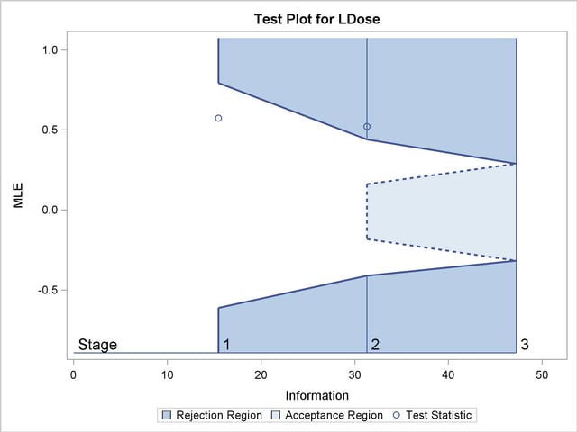
With the RCI option, the "Repeated Confidence Intervals" table in Output 78.8.16 displays repeated confidence intervals for the parameter. For a two-sided test, since the rejection lower repeated confidence limit  is greater than the null reference zero, the trial is stopped to reject the hypothesis.
With the PLOTS=RCI option, the "Repeated Confidence Intervals Plot" displays repeated confidence intervals for the parameter, as shown in Output 78.8.17. It shows that the null reference zero is inside the rejection repeated confidence interval at stage but outside the rejection repeated confidence interval at stage . This implies that the study stops at stage to reject the hypothesis.
Note that the hypothesis is accepted if at any stage, the acceptance repeated confidence interval falls within the interval  of the alternative references.
Copyright © 2009 by SAS Institute Inc., Cary, NC, USA. All rights reserved.