| The SEQDESIGN Procedure |
Example 77.5 Creating Designs Using Haybittle-Peto Methods
This example requests two 3-stage group sequential designs for normally distributed statistics. Each design uses a Haybittle-Peto method with a two-sided alternative and early stopping to reject the hypothesis. One design uses the specified interim boundary  values and derives the final-stage boundary value for the specified
  and
and  errors. The other design uses the specified boundary values and derives the overall and errors.
The following statements specify the interim boundary values and derive the final-stage boundary value for the specified  and
and  :
:
   ods graphics on;
   proc seqdesign altref=0.25
                  errspend
                  stopprob
                  plots=errspend
                  ;
      OneSidedPeto: design nstages=3
                    method=peto( z=3)
                    alt=upper   stop=reject
                    alpha=0.05  beta=0.10;
   run;
   ods graphics off;
The "Design Information" table in Output 77.5.1 displays design specifications and maximum information in percentage of its corresponding fixed-sample design.
| Design Information | |
|---|---|
| Statistic Distribution | Normal |
| Boundary Scale | Standardized Z |
| Alternative Hypothesis | Upper |
| Early Stop | Reject Null |
| Method | Haybittle-Peto |
| Boundary Key | Both |
| Alternative Reference | 0.25 |
| Number of Stages | 3 |
| Alpha | 0.05 |
| Beta | 0.1 |
| Power | 0.9 |
| Max Information (Percent of Fixed Sample) | 100.2466 |
| Max Information | 137.3592 |
| Null Ref ASN (Percent of Fixed Sample) | 100.1192 |
| Alt Ref ASN (Percent of Fixed Sample) | 87.35 |
The "Method Information" table in Output 77.5.2 displays the and errors and the derived drift parameter, which is the standardized alternative reference at the final stage.
With the STOPPROB option, the "Expected Cumulative Stopping Probabilities" table in Output 77.5.3 displays the expected stopping stage and cumulative stopping probability to reject the null hypothesis at each stage under various hypothetical references  , where
  is the alternative reference and
  are the default values in the CREF= option.
| Expected Cumulative Stopping Probabilities Reference = CRef * (Alt Reference) |
|||||
|---|---|---|---|---|---|
| CRef | Expected Stopping Stage |
Source | Stopping Probabilities | ||
| Stage_1 | Stage_2 | Stage_3 | |||
| 0.0000 | 2.996 | Reject Null | 0.00135 | 0.00246 | 0.05000 |
| 0.5000 | 2.941 | Reject Null | 0.01561 | 0.04372 | 0.42762 |
| 1.0000 | 2.614 | Reject Null | 0.09538 | 0.29057 | 0.90000 |
| 1.5000 | 1.944 | Reject Null | 0.32185 | 0.73442 | 0.99698 |
The "Boundary Information" table in Output 77.5.4 displays information level, alternative references, and boundary values. The default BOUNDARYSCALE=STDZ option specifies that the standardized scale be used to display the alternative references and boundary values. The resulting standardized alternative reference at stage  is given by
  , where
  is the alternative reference and
  is the information level at stage ,
  .
.
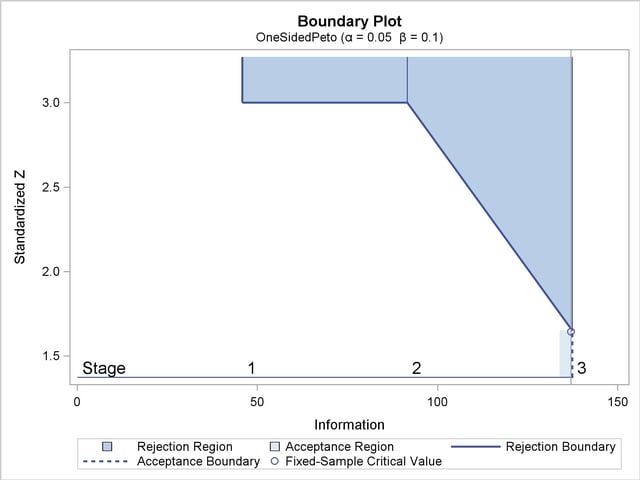
At each interim stage, if the standardized statistic  , the trial is stopped and the null hypothesis is rejected. If the statistic
  , the trial continues to the next stage. At the final stage, the null hypothesis is rejected if the statistic
  . Otherwise, the hypothesis is accepted. Note that the boundary values at the final stage,
  , are close to the critical values
  in the corresponding fixed-sample design.
The "Error Spending Information" in Output 77.5.5 displays cumulative error spending at each stage for each boundary. The stage  spending
  corresponds to the one-sided
  -value for a standardized statistic,
  .
.
With the specified ODS GRAPHICS ON statement, a detailed boundary plot with the rejection and acceptance regions is displayed by default, as shown in Output 77.5.6. With the STOP=REJECT option, the interim rejection boundaries are displayed.
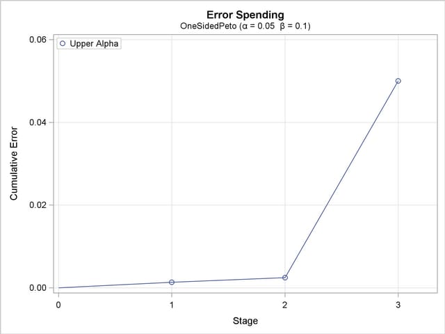
With the PLOTS=ERRSPEND option, the procedure displays a plot of error spending for each boundary, as shown in Output 77.5.7. The error spending values in the "Error Spending Information" in Output 77.5.4 are displayed in the plot. As expected, the error spending at each of the first two stages is small, with the standardized boundary value  .
.
The following statements specify the boundary values and derive the and errors from these completely specified boundary values:
   ods graphics on;
   proc seqdesign altref=0.25
                  maxinfo=200
                  errspend
                  stopprob
                  plots=errspend
                  ;
      OneSidedPeto: design nstages=3
                    method=peto(z=3 2.5 2)
                    alt=upper  stop=reject
                    boundarykey=none
                    ;
   run;
   ods graphics off;
The "Design Information" table in Output 77.5.8 displays design specifications and derived and error levels.
| Design Information | |
|---|---|
| Statistic Distribution | Normal |
| Boundary Scale | Standardized Z |
| Alternative Hypothesis | Upper |
| Early Stop | Reject Null |
| Method | Haybittle-Peto |
| Boundary Key | None |
| Alternative Reference | 0.25 |
| Number of Stages | 3 |
| Alpha | 0.02532 |
| Beta | 0.06035 |
| Power | 0.93965 |
| Max Information (Percent of Fixed Sample) | 101.6769 |
| Max Information | 200 |
| Null Ref ASN (Percent of Fixed Sample) | 101.3933 |
| Alt Ref ASN (Percent of Fixed Sample) | 73.74031 |
The "Method Information" table in Output 77.5.9 displays the and errors and the derived drift parameter for each boundary.
With the STOPPROB option, the "Expected Cumulative Stopping Probabilities" table in Output 77.5.10 displays the expected stopping stage and cumulative stopping probability to reject the null hypothesis at each stage under various hypothetical references , where is the alternative reference and are the default values in the CREF= option.
| Expected Cumulative Stopping Probabilities Reference = CRef * (Alt Reference) |
|||||
|---|---|---|---|---|---|
| CRef | Expected Stopping Stage |
Source | Stopping Probabilities | ||
| Stage_1 | Stage_2 | Stage_3 | |||
| 0.0000 | 2.992 | Reject Null | 0.00135 | 0.00702 | 0.02532 |
| 0.5000 | 2.826 | Reject Null | 0.02389 | 0.15030 | 0.41775 |
| 1.0000 | 2.176 | Reject Null | 0.16884 | 0.65544 | 0.93965 |
| 1.5000 | 1.508 | Reject Null | 0.52466 | 0.96708 | 0.99954 |
The "Boundary Information" table in Output 77.5.11 displays information level, alternative references, and boundary values.
The "Error Spending Information" in Output 77.5.12 displays cumulative error spending at each stage for each boundary. The first-stage spending corresponds to the one-sided -value for a standardized statistic, .
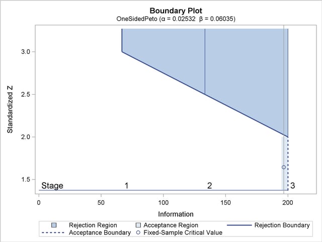
With the specified ODS GRAPHICS ON statement, a detailed boundary plot with the rejection and acceptance regions is displayed by default, as shown in Output 77.5.13. With the STOP=REJECT option, the interim rejection boundaries are displayed.
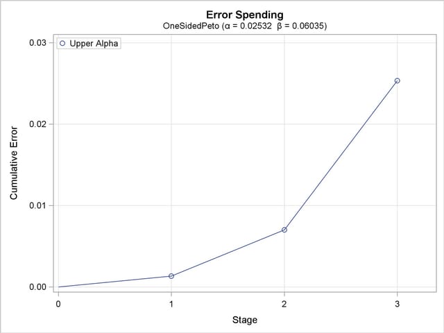
With the PLOTS=ERRSPEND option, the procedure displays a plot of error spending for each boundary, as shown in Output 77.5.14. The error spending values in the "Error Spending Information" table in Output 77.5.10 are displayed in the plot.
Copyright © 2009 by SAS Institute Inc., Cary, NC, USA. All rights reserved.