| The SEQDESIGN Procedure |
Example 77.2 Creating a One-Sided O’Brien-Fleming Design
This example demonstrates a group sequential design for a clinical study. A clinic is conducting a study on the effect of vitamin C supplements in treating flu symptoms. The study groups consist of patients in the clinic with their first sign of flu symptoms within the last 24 hours. These individuals are randomly assigned to either the control group, which receives the placebo pills, or the treatment group, which receives large doses of vitamin C supplements. At the end of a five-day period, the flu symptoms of each individual are recorded.
Suppose that from past experience,  of individuals experiencing flu symptoms have the symptoms disappeared within five days. The clinic wants to detect a
  symptoms disappearance with a high probability in the trial. A test that compares the proportions directly is to specify a null hypothesis
  with a Type I error probability level
  , where
  and
and  are the proportions of symptoms’ disappearance in the treatment group and control group, respectively. A one-sided alternative
  is also specified with a power of
  at
at  .
.
For a one-sided fixed-sample design, the critical value for the standardized  test statistic is given by
  . That is, at the end of study, if the test statistic
  , then the null hypothesis is rejected and the efficacy of vitamin C supplements is declared. Otherwise, the null hypothesis is not rejected and the effect of vitamin C supplements is not significant.
To achieve a power at for a fixed-sample design, the information required is given by
 |
With an equal sample size on the treatment and control groups,  , the sample size required for each group under
  is computed from the information
  :
:
 |
where  and
and  are proportions in the treatment and control groups under . That is,
 |
Thus,  individuals are required for each group in the fixed-sample study. See the section Test for the Difference between Two Binomial Proportions for a detailed derivation of these required sample sizes.
Instead of a fixed-sample design for the trial, a group sequential design is used to stop the trial early for ethical concerns of possible harm or an unexpected strong efficacy outcome of the new drug. It can also save time and resources in the process. The following statements invoke the SEQDESIGN procedure and request a four-stage group sequential design that uses an O’Brien-Fleming method for normally distributed statistics. The design uses a one-sided alternative hypothesis with early stopping to reject or accept  .
.
   ods graphics on;
   proc seqdesign altref=0.15
                  ;
      OneSidedOBrienFleming: design nstages=4
                             method=obf
                             alt=upper   stop=both
                             alpha=0.025 beta=0.10
                             ;
      samplesize model=twosamplefreq(nullprop=0.6 test=prop);
   ods output Boundary=Bnd_Prop;
   run;
   ods graphics off;
In a sequential design, a hypothesis can be rejected, accepted, or continued to the next time point at each interim stage. The STOP=BOTH option specifies early stopping to reject or accept the null hypothesis. The "Design Information," "Method Information," and "Boundary Information" tables are displayed by default.
The "Design Information" table in Output 77.2.1 displays design specifications and derived statistics such as power and maximum information. With a specified alternative reference, ALTREF=0.15, the maximum information  is derived.
| Design Information | |
|---|---|
| Statistic Distribution | Normal |
| Boundary Scale | Standardized Z |
| Alternative Hypothesis | Upper |
| Early Stop | Accept/Reject Null |
| Method | O'Brien-Fleming |
| Boundary Key | Both |
| Alternative Reference | 0.15 |
| Number of Stages | 4 |
| Alpha | 0.025 |
| Beta | 0.1 |
| Power | 0.9 |
| Max Information (Percent of Fixed Sample) | 107.6741 |
| Max Information | 502.8343 |
| Null Ref ASN (Percent of Fixed Sample) | 61.12891 |
| Alt Ref ASN (Percent of Fixed Sample) | 75.89782 |
The Max Information (Percent Fixed-Sample) is the ratio in percentage between the maximum information for the group sequential design and the information required for a corresponding fixed-sample design:
 |
That is, if the group sequential trial does not stop at any interim stages, the information needed is  more than is needed for the corresponding fixed-sample design. For a two-sample test for binomial proportions, the information is proportional to the sample size. Thus, more observations are needed for the group sequential trial.
The Null Ref ASN (Percent Fixed-Sample) is the ratio in percentage between the expected sample size required under the null hypothesis for the group sequential design and the sample size required for the corresponding fixed-sample design. With a ratio of  , the expected sample size for the group sequential trial under the null hypothesis is of the sample size in the corresponding fixed-sample design.
Similarly, the Alt Ref ASN (Percent Fixed-Sample) is the ratio in percentage between the expected sample size required under the alternative hypothesis for the group sequential design and the sample size required for the corresponding fixed-sample design. With a ratio of  , the expected sample size for the group sequential trial under the alternative hypothesis is of the sample size in the corresponding fixed-sample design.
For a one-sided design with an upper alternative and early stopping to reject or accept the null hypothesis, upper  and
and  boundaries are created. The "Method Information" table in Output 77.2.2 displays the Type I error probability , the Type II error probability , and the derived drift parameter. The drift parameter is the standardized reference improvement between the alternative and null hypotheses at the final stage. It is also the standardized alternative reference at the final stage if the null reference is zero.
With the METHOD=OBF option, the O’Brien-Fleming method is used for each boundary. The O’Brien-Fleming method is one of the unified family methods, and the "Method Information" table displays the corresponding parameter  in the unified family method. The table also displays the critical values
  for the boundary and
  for the boundary. These critical values are used to create the boundary values. With the default BOUNDARYSCALE=STDZ option, the boundaries are displayed with the standardized statistic scale.
The "Boundary Information" table in Output 77.2.3 displays information level, alternative reference, and boundary values at each stage. The default BOUNDARYSCALE=STDZ option specifies that the standardized scale be used to display the alternative references and boundary values. The resulting standardized alternative reference at stage  is given by
  , where
  is the alternative reference and
  is the information level at stage ,
  .
.
| Boundary Information (Standardized Z Scale) Null Reference = 0 |
||||||
|---|---|---|---|---|---|---|
| _Stage_ | Alternative | Boundary Values | ||||
| Information Level | Reference | Upper | ||||
| Proportion | Actual | N | Upper | Beta | Alpha | |
| 1 | 0.2500 | 125.7086 | 107.4808 | 1.68180 | -1.08860 | 3.95679 |
| 2 | 0.5000 | 251.4171 | 214.9617 | 2.37842 | 0.41946 | 2.79788 |
| 3 | 0.7500 | 377.1257 | 322.4425 | 2.91296 | 1.31347 | 2.28446 |
| 4 | 1.0000 | 502.8343 | 429.9233 | 3.36360 | 1.97840 | 1.97840 |
By default, equally spaced information levels are used. An information proportion is the proportion of maximum information available at each stage. With the derived maximum information, the actual information level at each stage is also displayed. With the SAMPLESIZE statement, the required sample size  is also displayed under the heading "Information Level."
At each interim stage, if the standardized test statistic is larger than or equal to the corresponding upper boundary, then the hypothesis  is rejected. If the test statistic is less than the corresponding upper boundary, then the trial is stopped and the hypothesis is accepted. Otherwise, the process continues to the next stage. At the final stage, stage
  , the trial stops and the hypothesis is rejected if the standardized statistic
  . Otherwise, the trial is accepted.
The ODS OUTPUT statement with the BOUNDARY=BND_PROP option creates an output data set that contains the resulting boundary information. After the actual data from the clinical trial are collected and analyzed at each stage with a procedure such as PROC GENMOD, the SEQTEST procedure is used to test the resulting statistics at stage  with the boundary information stored in the BOUND_PROP data set.
With the specified ODS GRAPHICS ON statement, a detailed boundary plot with the rejection and acceptance regions is displayed by default, as shown in Output 77.2.4.
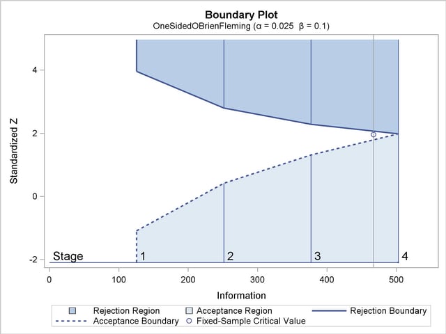
The horizontal axis indicates the information levels for the design. The stages are indicated by vertical lines with accompanying stage numbers. If at any stage a test statistic is in a rejection region, the trial stops and the hypothesis is rejected. If a test statistic is in an acceptance region, then the trial also stops and the hypothesis is accepted. If the statistic is not in a rejection region or an acceptance region, the trial continues to the next stage. The boundary plot also displays the information level and critical value for the corresponding fixed-sample design.
The SEQDESIGN procedure derives the drift parameter  , where
  is the alternative reference and is the maximum information. If either or is specified, the other can be derived. With the SAMPLESIZE statement, the maximum information is used to compute the required sample size for the study.
The "Sample Size Summary" table in Output 77.2.5 displays parameters for the sample size computation. With the MODEL=TWOSAMPLEFREQ( NULLPROP=0.6 TEST=PROP) option in the SAMPLESIZE statement, the total sample size in each group for testing the difference between two proportions is computed. With the default REF=PROP option, the required sample sizes are computed under the alternative hypothesis. That is,
 |
where  and
and  are the proportions in the control and treatment groups, respectively, under the alternative hypothesis . See the section Test for the Difference between Two Binomial Proportions for a detailed description of these parameters.
The "Sample Sizes (N)" table in Output 77.2.6 displays the required sample sizes at each stage, in both fractional and integer numbers. The derived fractional sample sizes are under the heading "Fractional N." These sample sizes are rounded up to integers under the heading "Ceiling N." In practice, integer sample sizes are used, and the resulting information levels increase slightly. Thus,  ,
,  ,
,  , and
, and  individuals are needed in each group for the four stages, respectively.
| Sample Sizes (N) Two-Sample Z Test for Proportion Difference |
||||||||
|---|---|---|---|---|---|---|---|---|
| _Stage_ | Fractional N | Ceiling N | ||||||
| N | N(Grp 1) | N(Grp 2) | Information | N | N(Grp 1) | N(Grp 2) | Information | |
| 1 | 107.48 | 53.74 | 53.74 | 125.7 | 108 | 54 | 54 | 126.3 |
| 2 | 214.96 | 107.48 | 107.48 | 251.4 | 216 | 108 | 108 | 252.6 |
| 3 | 322.44 | 161.22 | 161.22 | 377.1 | 324 | 162 | 162 | 378.9 |
| 4 | 429.92 | 214.96 | 214.96 | 502.8 | 430 | 215 | 215 | 502.9 |
Copyright © 2009 by SAS Institute Inc., Cary, NC, USA. All rights reserved.