| The ROBUSTREG Procedure |
| High Breakdown Value Estimation |
The breakdown value of an estimator is defined as the smallest fraction of contamination that can cause the estimator to take on values arbitrarily far from its value on the uncontamined data. The breakdown value of an estimator can be used as a measure of the robustness of the estimator. Rousseeuw and Leroy (1987) and others introduced the following high breakdown value estimators for linear regression.
LTS Estimate
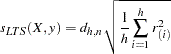
The least trimmed squares (LTS) estimate proposed by Rousseeuw (1984) is defined as the  -vector
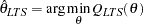 |
where
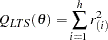 |
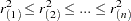 are the ordered squared residuals
 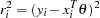 ,
,  , and
, and  is defined in the range
  .
.
You can specify the parameter with the H= option in the PROC statement. By default,  . The breakdown value is
  for the LTS estimate.
The ROBUSTREG procedure computes LTS estimates by using the FAST-LTS algorithm of Rousseeuw and Van Driessen (2000). The estimates are often used to detect outliers in the data, which are then downweighted in the resulting weighted LS regression.
Algorithm
Least trimmed squares (LTS) regression is based on the subset of observations (out of a total of  observations) whose least squares fit possesses the smallest sum of squared residuals. The coverage
  can be set between
  and . The LTS method was proposed by Rousseeuw (1984, p. 876) as a highly robust regression estimator with breakdown value
  . The ROBUSTREG procedure uses the FAST-LTS algorithm given by Rousseeuw and Van Driessen (2000). The intercept adjustment technique is also used in this implementation. However, because this adjustment is expensive to compute, it is optional. You can use the IADJUST option in the PROC statement to request or suppress the intercept adjustment. By default, PROC ROBUSTREG does intercept adjustment for data sets with fewer than 10000 observations. The steps of the algorithm are described briefly as follows. Refer to Rousseeuw and Van Driessen (2000) for details.
The default
is  , where
  is the number of independent variables. You can specify any integer with
  with the H= option in the MODEL statement. The breakdown value for LTS, , is reported. The default is a good compromise between breakdown value and statistical efficiency.
 If
 (single regressor), the procedure uses the exact algorithm of Rousseeuw and Leroy (1987, p. 172).
 If
 , the procedure uses the following algorithm. If
  , where
  is the size of the subgroups (you can specify by using the SUBGROUPSIZE= option in the PROC statement; by default,
  ), draw a random -subset and compute the regression coefficients by using these points (if the regression is degenerate, draw another -subset). Compute the absolute residuals for all observations in the data set, and select the first points with smallest absolute residuals. From this selected -subset, carry out
  C-steps (Concentration step; see Rousseeuw and Van Driessen (2000) for details. You can specify with the CSTEP= option in the PROC statement; by default,
  ). Redraw -subsets and repeat the preceding computing procedure
  times, and then find the
  (at most) solutions with the lowest sums of squared residuals. can be specified with the NREP= option in the PROC statement. By default, NREP=
 . For small and , all
  subsets are used and the NREP= option is ignored (Rousseeuw and Hubert 1996). can be specified with the NBEST= option in the PROC statement. By default, NBEST=10. For each of these best solutions, take C-steps until convergence and find the best final solution.
 If
 , construct 5 disjoint random subgroups with size
  . If
. If  , the data are split into at most four subgroups with or more observations in each subgroup, so that each observation belongs to a subgroup and the subgroups have roughly the same size. Let
  denote the number of subgroups. Inside each subgroup, repeat the procedure in step 3
  times and keep the best solutions. Pool the subgroups, yielding the merged set of size
  . In the merged set, for each of the
  best solutions, carry out C-steps by using and
  and keep the best solutions. In the full data set, for each of these best solutions, take C-steps by using and until convergence and find the best final solution.
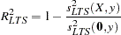
The robust version of  for the LTS estimate is defined as
 |
for models with the intercept term and as
 |
for models without the intercept term, where
 |
 is a preliminary estimate of the parameter
  in the distribution function
  .
.
Here  is chosen to make consistent, assuming a Gaussian model. Specifically,
 |
 |
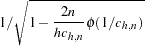 |
|||
 |
|
 |
with  and
and  being the distribution function and the density function of the standard normal distribution, respectively.
Final Weighted Scale Estimator
The ROBUSTREG procedure displays two scale estimators, and Wscale. The estimator Wscale is a more efficient scale estimator based on the preliminary estimate , and it is defined as
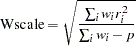 |
where
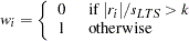 |
You can specify  with the CUTOFF= option in the MODEL statement. By default,
  .
.
S Estimate
The S estimate proposed by Rousseeuw and Yohai (1984) is defined as the -vector
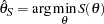 |
where the dispersion  is the solution of
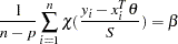 |
Here  is set to
  such that
  and
and  are asymptotically consistent estimates of
  and for the Gaussian regression model. The breakdown value of the S estimate is
 |
The ROBUSTREG procedure provides two choices for  : Tukey’s bisquare function and Yohai’s optimal function.
Tukey’s bisquare function, which you can specify with the option CHIF=TUKEY, is
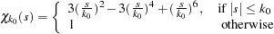 |
The constant  controls the breakdown value and efficiency of the S estimate. If you specify the efficiency by using the EFF= option, you can determine the corresponding . The default is 2.9366 such that the breakdown value of the S estimate is 0.25 with a corresponding asymptotic efficiency for the Gaussian model of
  .
.
The Yohai function, which you can specify with the option CHIF=YOHAI, is
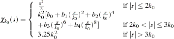 |
where  ,
,  ,
,  ,
,  , and
, and  . If you specify the efficiency by using the EFF= option, you can determine the corresponding . By default, is set to 0.7405 such that the breakdown value of the S estimate is 0.25 with a corresponding asymptotic efficiency for the Gaussian model of
  .
.
Algorithm
The ROBUSTREG procedure implements the algorithm by Marazzi (1993) for the S estimate, which is a refined version of the algorithm proposed by Ruppert (1992). The refined algorithm is briefly described as follows.
Initialize  .
.
Draw a random
 -subset of the total observations and compute the regression coefficients by using these observations (if the regression is degenerate, draw another
  -subset), where
  can be specified with the SUBSIZE= option. By default,
  .
. Compute the residuals:
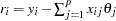 for . If , set
  ; if
; if  , set
, set 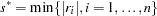 ;
;
while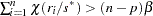 , set
, set  ; go to step 3.
If and
and  , go to step 3; otherwise, go to step 5.
 Solve for
 the equation
using an iterative algorithm.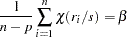
If
and  , go to step 5. Otherwise, set
  and
and  . If
. If  , return
  and
and  ; otherwise, go to step 5.
 If
 , set
, set  and return to step 1; otherwise, return and .
The ROBUSTREG procedure does the following refinement step by default. You can request that this refinement not be done by using the NOREFINE option in the PROC statement.
Let
 . Using the values and from the previous steps, compute M estimates
  and
and  of and with the setup for M estimation in the section M Estimation. If
  , give a warning and return and ; otherwise, return and .
You can specify  with the TOLERANCE= option; by default, TOLERANCE=0.001. Alternately, you can specify
  with the NREP= option. You can also use the options NREP=NREP0 or NREP=NREP1 to determine according to the following table. NREP=NREP0 is set as the default.
P |
NREP0 |
NREP1 |
1 |
150 |
500 |
2 |
300 |
1000 |
3 |
400 |
1500 |
4 |
500 |
2000 |
5 |
600 |
2500 |
6 |
700 |
3000 |
7 |
850 |
3000 |
8 |
1250 |
3000 |
9 |
1500 |
3000 |
>9 |
1500 |
3000 |
 and Deviance
The robust version of for the S estimate is defined as
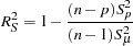 |
for the model with the intercept term and
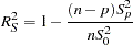 |
for the model without the intercept term, where  is the S estimate of the scale in the full model,
  is the S estimate of the scale in the regression model with only the intercept term, and
  is the S estimate of the scale without any regressor. The deviance
  is defined as the optimal value of the objective function on the
  scale:
 |
Asymptotic Covariance and Confidence Intervals
Since the S estimate satisfies the first-order necessary conditions as the M estimate, it has the same asymptotic covariance as that of the M estimate. All three estimators of the asymptotic covariance for the M estimate in the section Asymptotic Covariance and Confidence Intervals can be used for the S estimate. Besides, the weighted covariance estimator H4 described in the section Asymptotic Covariance and Confidence Intervals is also available and is set as the default. Confidence intervals for estimated parameters are computed from the diagonal elements of the estimated asymptotic covariance matrix.
Copyright © 2009 by SAS Institute Inc., Cary, NC, USA. All rights reserved.