| The POWER Procedure |
Analyses in the PAIREDMEANS Statement
Paired t Test (TEST=DIFF)
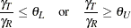
The hypotheses for the paired  test are
 |
 |
|||
 |
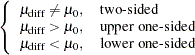 |
The test assumes normally distributed data and requires  . The test statistics are
 |
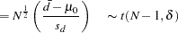 |
|||
 |
 |
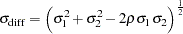
where  and
and  are the sample mean and standard deviation of the differences and
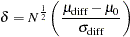 |
and
 |
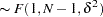
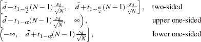
The test is
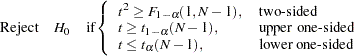 |
Exact power computations for tests are given in O’Brien and Muller (1993, Section 8.2.2):
 |
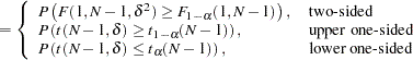 |
Paired t Test for Mean Ratio with Lognormal Data (TEST=RATIO)
The lognormal case is handled by reexpressing the analysis equivalently as a normality-based test on the log-transformed data, by using properties of the lognormal distribution as discussed in Johnson, Kotz, and Balakrishnan (1994, Chapter 14). The approaches in the section Paired t Test (TEST=DIFF) then apply.
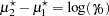
In contrast to the usual test on normal data, the hypotheses with lognormal data are defined in terms of geometric means rather than arithmetic means.
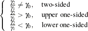
The hypotheses for the paired test with lognormal pairs  are
are
|
 |
|||
|
 |
Let  ,
,  ,
,  ,
,  , and
, and  be the (arithmetic) means, standard deviations, and correlation of the bivariate normal distribution of the log-transformed data
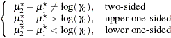
  . The hypotheses can be rewritten as follows:
|
 |
|||
|
 |
where
 |
 |
|||
 |
 |
|||
 |
 |
|||
 |
 |
|||
 |
 |
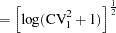
and  ,
,  , and
, and  are the coefficients of variation and the correlation of the original untransformed pairs . The conversion from to is shown in Jones and Miller (1966).
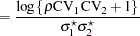
The test assumes lognormally distributed data and requires . The power is
 |
where
 |
and
 |
Additive Equivalence Test for Mean Difference with Normal Data (TEST=EQUIV_DIFF)
The hypotheses for the equivalence test are
|
 |
|||
|
 |
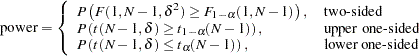
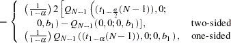
The analysis is the two one-sided tests (TOST) procedure of Schuirmann (1987). The test assumes normally distributed data and requires . Phillips (1990) derives an expression for the exact power assuming a two-sample balanced design; the results are easily adapted to a paired design:
|
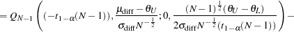 |
|||
 |
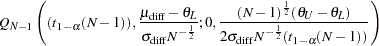 |
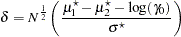
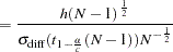
where
|
and  is Owen’s Q function, defined in the section Common Notation.
Multiplicative Equivalence Test for Mean Ratio with Lognormal Data (TEST=EQUIV_RATIO)
The lognormal case is handled by reexpressing the analysis equivalently as a normality-based test on the log-transformed data, by using properties of the lognormal distribution as discussed in Johnson, Kotz, and Balakrishnan (1994, Chapter 14). The approaches in the section Additive Equivalence Test for Mean Difference with Normal Data (TEST=EQUIV_DIFF) then apply.
In contrast to the additive equivalence test on normal data, the hypotheses with lognormal data are defined in terms of geometric means rather than arithmetic means.
The hypotheses for the equivalence test are
|
 |
|||
|
 |
 |
The analysis is the two one-sided tests (TOST) procedure of Schuirmann (1987) on the log-transformed data. The test assumes lognormally distributed data and requires . Diletti, Hauschke, and Steinijans (1991) derive an expression for the exact power assuming a crossover design; the results are easily adapted to a paired design:
|
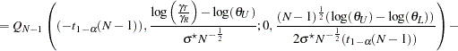 |
|||
|
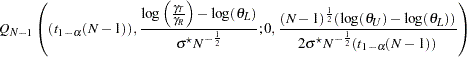 |
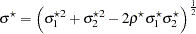
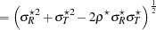
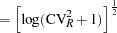
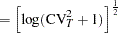
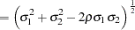
where  is the standard deviation of the differences between the log-transformed pairs (in other words, the standard deviation of
  , where
  and
and  are observations from the treatment and reference, respectively), computed as
 |
 |
|||
 |
 |
|||
 |
 |
|||
|
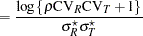 |
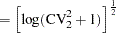
where  ,
,  , and are the coefficients of variation and the correlation of the original untransformed pairs
  , and is Owen’s Q function. The conversion from to is shown in Jones and Miller (1966), and Owen’s Q function is defined in the section Common Notation.
Confidence Interval for Mean Difference (CI=DIFF)
This analysis of precision applies to the standard -based confidence interval:
 |
where and are the sample mean and standard deviation of the differences. The "half-width" is defined as the distance from the point estimate to a finite endpoint,
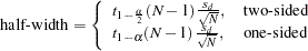 |
A "valid" conference interval captures the true mean difference. The exact probability of obtaining at most the target confidence interval half-width  , unconditional or conditional on validity, is given by Beal (1989):
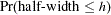 |
 |
|||
 |
 |
where
 |
 |
|||
 |
 |
|||
 |
 |
and is Owen’s Q function, defined in the section Common Notation.
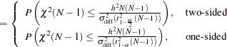
A "quality" confidence interval is both sufficiently narrow (half-width  ) and valid:
 |
 |
|||
|
 |
Copyright © 2009 by SAS Institute Inc., Cary, NC, USA. All rights reserved.