| The PHREG Procedure |
Example 64.10 Analysis of Recurrent Events Data
Recurrent events data consist of times to a number of repeated events for each sample unit—for example, times of recurrent episodes of a disease in patients. Various ways of analyzing recurrent events data are described in the section Analysis of Multivariate Failure Time Data. The bladder cancer data listed in Wei, Lin, and Weissfeld (1989) are used here to illustrate these methods.
The data consist of 86 patients with superficial bladder tumors, which were removed when the patients entered the study. Of these patients, 48 were randomized into the placebo group, and 38 were randomized into the group receiving thiotepa. Many patients had multiple recurrences of tumors during the study, and new tumors were removed at each visit. The data set contains the first four recurrences of the tumor for each patient, and each recurrence time was measured from the patient’s entry time into the study.
The data consist of the following eight variables:
Trt, treatment group (1=placebo and 2=thiotepa)
Time, follow-up time
Number, number of initial tumors
Size, initial tumor size
T1, T2, T3, and T4, times of the four potential recurrences of the bladder tumor. A patient with only two recurrences has missing values in T3 and T4.
In the data set Bladder, four observations are created for each patient, one for each of the four potential tumor recurrences. In addition to values of Trt, Number, and Size for the patient, each observation contains the following variables:
ID, patient’s identification (which is the sequence number of the subject)
Visit, visit number (with value
 for the th potential tumor recurrence)
 TStart, time of the (
–1)th recurrence for Visit=, or the entry time 0 if VISIT=1, or the follow-up time if the (–1)th recurrence does not occur TStop, time of the
th recurrence if Visit= or follow-up time if the th recurrence does not occur Status, event status of TStop (1=recurrence and 0=censored)
For instance, a patient with only one recurrence time at month 6 who was followed until month 10 will have values for Visit, TStart, TStop, and Status of (1,0,6,1), (2,6,10,0), (3,10,10,0), and (4,10,10,0), respectively. The last two observations are redundant for the intensity model and the proportional means model, but they are important for the analysis of the marginal Cox models. If the follow-up time is beyond the time of the fourth tumor recurrence, it is tempting to create a fifth observation with the time of the fourth tumor recurrence as the TStart value, the follow-up time as the TStop value, and a Status value of 0. However, Therneau and Grambsch (2000, Section 8.5) have warned against incorporating such observations into the analysis.
The following SAS statements create the data set Bladder:
   data Bladder;
      keep ID TStart TStop Status Trt Number Size Visit;
      retain ID TStart 0;
      array tt T1-T4;
      infile datalines missover;
      input Trt Time Number Size T1-T4;
      ID + 1;
      TStart=0;
      do over tt;
         Visit=_i_;
         if tt = . then do;
            TStop=Time;
            Status=0;
         end;
         else do;
            TStop=tt;
            Status=1;
         end;
         output;
         TStart=TStop;
      end;
      if (TStart < Time) then delete;
      datalines;
   1       0       1     1
   1       1       1     3
   1       4       2     1
   1       7       1     1
   1       10      5     1
   1       10      4     1   6
   1       14      1     1
   1       18      1     1
   1       18      1     3   5
   1       18      1     1   12  16
   1       23      3     3
   1       23      1     3   10  15
   1       23      1     1   3   16  23
   1       23      3     1   3   9   21
   1       24      2     3   7   10  16  24
   1       25      1     1   3   15  25
   1       26      1     2
   1       26      8     1   1
   1       26      1     4   2   26
   1       28      1     2   25
   1       29      1     4
   1       29      1     2
   1       29      4     1
   1       30      1     6   28  30
   1       30      1     5   2   17  22
   1       30      2     1   3   6   8   12
   1       31      1     3   12  15  24
   1       32      1     2
   1       34      2     1
   1       36      2     1
   1       36      3     1   29
   1       37      1     2
   1       40      4     1   9   17  22  24
   1       40      5     1   16  19  23  29
   1       41      1     2
   1       43      1     1   3
   1       43      2     6   6
   1       44      2     1   3   6   9
   1       45      1     1   9   11  20  26
   1       48      1     1   18
   1       49      1     3
   1       51      3     1   35
   1       53      1     7   17
   1       53      3     1   3   15  46  51
   1       59      1     1
   1       61      3     2   2   15  24  30
   1       64      1     3   5   14  19  27
   1       64      2     3   2   8   12  13
   2       1       1     3
   2       1       1     1
   2       5       8     1   5
   2       9       1     2
   2       10      1     1
   2       13      1     1
   2       14      2     6   3
   2       17      5     3   1   3   5   7
   2       18      5     1
   2       18      1     3   17
   2       19      5     1   2
   2       21      1     1   17  19
   2       22      1     1
   2       25      1     3
   2       25      1     5
   2       25      1     1
   2       26      1     1   6   12  13
   2       27      1     1   6
   2       29      2     1   2
   2       36      8     3   26  35
   2       38      1     1
   2       39      1     1   22  23  27  32
   2       39      6     1   4   16  23  27
   2       40      3     1   24  26  29  40
   2       41      3     2
   2       41      1     1
   2       43      1     1   1   27
   2       44      1     1
   2       44      6     1   2   20  23  27
   2       45      1     2
   2       46      1     4   2
   2       46      1     4
   2       49      3     3
   2       50      1     1
   2       50      4     1   4   24  47
   2       54      3     4
   2       54      2     1   38
   2       59      1     3
   ;
   run;
First, consider fitting the intensity model (Andersen and Gill; 1982) and the proportional means model (Lin et al.; 2000). The counting process style of input is used in the PROC PHREG specification. For the proportional means model, inference is based on the robust sandwich covariance estimate, which is requested by the COVB(AGGREGATE) option in the PROC PHREG statement. The COVM option is specified for the analysis of the intensity model to use the model-based covariance estimate. Note that some of the observations in the data set Bladder have a degenerated interval of risk. The presence of these observations does not affect the results of the analysis since none of these observations are included in any of the risk sets. However, the procedure will run more efficiently without these observations; consequently, in the following SAS statements, the WHERE clause is used to eliminate these redundant observations:
   title 'Intensity Model and Proportional Means Model';
   proc phreg data=Bladder covm covs(aggregate);
      model (TStart, TStop) * Status(0) = Trt Number Size;
      id id;
      where TStart < TStop;
   run;
Results of fitting the intensity model and the proportional means model are shown in Output 64.10.1 and Output 64.10.2, respectively. The robust sandwich standard error estimate for Trt is larger than its model-based counterpart, rendering the effect of thiotepa less significant in the proportional means model ( =0.0747) than in the intensity model (=0.0215).
| Analysis of Maximum Likelihood Estimates | ||||||
|---|---|---|---|---|---|---|
| with Model-Based Variance Estimate | ||||||
| Parameter | DF | Parameter Estimate |
Standard Error |
Chi-Square | Pr > ChiSq | Hazard Ratio |
| Trt | 1 | -0.45979 | 0.19996 | 5.2873 | 0.0215 | 0.631 |
| Number | 1 | 0.17165 | 0.04733 | 13.1541 | 0.0003 | 1.187 |
| Size | 1 | -0.04256 | 0.06903 | 0.3801 | 0.5375 | 0.958 |
| Analysis of Maximum Likelihood Estimates | |||||||
|---|---|---|---|---|---|---|---|
| with Sandwich Variance Estimate | |||||||
| Parameter | DF | Parameter Estimate |
Standard Error |
StdErr Ratio |
Chi-Square | Pr > ChiSq | Hazard Ratio |
| Trt | 1 | -0.45979 | 0.25801 | 1.290 | 3.1757 | 0.0747 | 0.631 |
| Number | 1 | 0.17165 | 0.06131 | 1.296 | 7.8373 | 0.0051 | 1.187 |
| Size | 1 | -0.04256 | 0.07555 | 1.094 | 0.3174 | 0.5732 | 0.958 |
Next, consider the conditional models of Prentice, Williams, and Peterson (1981). In the PWP models, the risk set for the (+1)th recurrence is restricted to those patients who have experienced the first recurrences. For example, a patient who experienced only one recurrence is an event observation for the first recurrence; this patient is a censored observation for the second recurrence and should not be included in the risk set for the third or fourth recurrence. The following DATA step eliminates those observations that should not be in the risk sets, forming a new input data set (named Bladder2) for fitting the PWP models. The variable Gaptime, representing the gap times between successive recurrences, is also created.
   data Bladder2(drop=LastStatus);
       retain LastStatus;
       set Bladder;
       by ID;
       if first.id then LastStatus=1;
       if (Status=0 and LastStatus=0) then delete;
       LastStatus=Status;
       Gaptime=Tstop-Tstart;
   run;
The following statements fit the PWP total time model. The variables Trt1, Trt2, Trt3, and Trt4 are visit-specific variables for Trt; the variables Number1, Number2, Numvber3, and Number4 are visit-specific variables for Number; and the variables Size1, Size2, Size3, and Size4 are visit-specific variables for Size.
   title 'PWP Total Time Model with Noncommon Effects';
   proc phreg data=Bladder2;
      model (TStart,Tstop) * Status(0) = Trt1-Trt4 Number1-Number4
                                         Size1-Size4;
      Trt1= Trt * (Visit=1);
      Trt2= Trt * (Visit=2);
      Trt3= Trt * (Visit=3);
      Trt4= Trt * (Visit=4);
      Number1= Number * (Visit=1);
      Number2= Number * (Visit=2);
      Number3= Number * (Visit=3);
      Number4= Number * (Visit=4);
      Size1= Size * (Visit=1);
      Size2= Size * (Visit=2);
      Size3= Size * (Visit=3);
      Size4= Size * (Visit=4);
      strata Visit;
   run;
Results of the analysis of the PWP total time model are shown in Output 64.10.3. There is no significant treatment effect on the total time in any of the four tumor recurrences.
| Summary of the Number of Event and Censored Values | |||||
|---|---|---|---|---|---|
| Stratum | Visit | Total | Event | Censored | Percent Censored |
| 1 | 1 | 85 | 47 | 38 | 44.71 |
| 2 | 2 | 46 | 29 | 17 | 36.96 |
| 3 | 3 | 27 | 22 | 5 | 18.52 |
| 4 | 4 | 20 | 14 | 6 | 30.00 |
| Total | 178 | 112 | 66 | 37.08 | |
| Analysis of Maximum Likelihood Estimates | ||||||
|---|---|---|---|---|---|---|
| Parameter | DF | Parameter Estimate |
Standard Error |
Chi-Square | Pr > ChiSq | Hazard Ratio |
| Trt1 | 1 | -0.51757 | 0.31576 | 2.6868 | 0.1012 | 0.596 |
| Trt2 | 1 | -0.45967 | 0.40642 | 1.2792 | 0.2581 | 0.631 |
| Trt3 | 1 | 0.11700 | 0.67183 | 0.0303 | 0.8617 | 1.124 |
| Trt4 | 1 | -0.04059 | 0.79251 | 0.0026 | 0.9592 | 0.960 |
| Number1 | 1 | 0.23605 | 0.07607 | 9.6287 | 0.0019 | 1.266 |
| Number2 | 1 | -0.02044 | 0.09052 | 0.0510 | 0.8213 | 0.980 |
| Number3 | 1 | 0.01219 | 0.18208 | 0.0045 | 0.9466 | 1.012 |
| Number4 | 1 | 0.18915 | 0.24443 | 0.5989 | 0.4390 | 1.208 |
| Size1 | 1 | 0.06790 | 0.10125 | 0.4498 | 0.5024 | 1.070 |
| Size2 | 1 | -0.15425 | 0.12300 | 1.5728 | 0.2098 | 0.857 |
| Size3 | 1 | 0.14891 | 0.26299 | 0.3206 | 0.5713 | 1.161 |
| Size4 | 1 | 0.0000732 | 0.34297 | 0.0000 | 0.9998 | 1.000 |
The following statements fit the PWP gap-time model:
   title 'PWP Gap-Time Model with Noncommon Effects';
   proc phreg data=Bladder2;
      model Gaptime * Status(0) = Trt1-Trt4 Number1-Number4
                                  Size1-Size4;
      Trt1= Trt * (Visit=1);
      Trt2= Trt * (Visit=2);
      Trt3= Trt * (Visit=3);
      Trt4= Trt * (Visit=4);
      Number1= Number * (Visit=1);
      Number2= Number * (Visit=2);
      Number3= Number * (Visit=3);
      Number4= Number * (Visit=4);
      Size1= Size * (Visit=1);
      Size2= Size * (Visit=2);
      Size3= Size * (Visit=3);
      Size4= Size * (Visit=4);
      strata Visit;
   run;
Results of the analysis of the PWP gap-time model are shown in Output 64.10.4. Note that the regression coefficients for the first tumor recurrence are the same as those of the total time model, since the total time and the gap time are the same for the first recurrence. There is no significant treatment effect on the gap times for any of the four tumor recurrences.
| Analysis of Maximum Likelihood Estimates | ||||||
|---|---|---|---|---|---|---|
| Parameter | DF | Parameter Estimate |
Standard Error |
Chi-Square | Pr > ChiSq | Hazard Ratio |
| Trt1 | 1 | -0.51757 | 0.31576 | 2.6868 | 0.1012 | 0.596 |
| Trt2 | 1 | -0.25911 | 0.40511 | 0.4091 | 0.5224 | 0.772 |
| Trt3 | 1 | 0.22105 | 0.54909 | 0.1621 | 0.6873 | 1.247 |
| Trt4 | 1 | -0.19498 | 0.64184 | 0.0923 | 0.7613 | 0.823 |
| Number1 | 1 | 0.23605 | 0.07607 | 9.6287 | 0.0019 | 1.266 |
| Number2 | 1 | -0.00571 | 0.09667 | 0.0035 | 0.9529 | 0.994 |
| Number3 | 1 | 0.12935 | 0.15970 | 0.6561 | 0.4180 | 1.138 |
| Number4 | 1 | 0.42079 | 0.19816 | 4.5091 | 0.0337 | 1.523 |
| Size1 | 1 | 0.06790 | 0.10125 | 0.4498 | 0.5024 | 1.070 |
| Size2 | 1 | -0.11636 | 0.11924 | 0.9524 | 0.3291 | 0.890 |
| Size3 | 1 | 0.24995 | 0.23113 | 1.1695 | 0.2795 | 1.284 |
| Size4 | 1 | 0.03557 | 0.29043 | 0.0150 | 0.9025 | 1.036 |
You can fit the PWP total time model with common effects by using the following SAS statements. However, the analysis is not shown here.
   title2 'PWP Total Time Model with Common Effects';
   proc phreg data=Bladder2;
      model (tstart,tstop) * status(0) = Trt Number Size;
      strata Visit;
   run;
You can fit the PWP gap-time model with common effects by using the following statements. Again, the analysis is not shown here.
   title2 'PWP Gap Time Model with Common Effects';
   proc phreg data=Bladder2;
      model Gaptime * Status(0) = Trt Number Size;
      strata Visit;
   run;
Recurrent events data are a special case of multiple events data in which the recurrence times are regarded as multivariate failure times and the marginal approach of Wei, Lin, and Weissfeld (1989) can be used. WLW fits a Cox model to each of the component times and makes statistical inference of the regression parameters based on a robust sandwich covariance matrix estimate. No specific correlation structure is imposed on the multivariate failure times. For the th marginal model, let  denote the row vector of regression parameters, let
  denote the maximum likelihood estimate of , let
  denote the covariance matrix obtained by inverting the observed information matrix, and let
  denote the matrix of score residuals. WLW showed that the joint distribution of
  can be approximated by a multivariate normal distribution with mean vector
  and robust covariance matrix
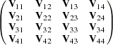 |
with the submatrix  given by
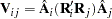 |
In this example, there are four marginal proportional hazards models, one for each potential recurrence time. Instead of fitting one model at a time, you can fit all four marginal models in one analysis by using the STRATA statement and model-specific covariates as in the following statements. Using Visit as the STRATA variable on the input data set Bladder, PROC PHREG simultaneously fits all four marginal models, one for each Visit value. The COVS(AGGREGATE) option is specified to compute the robust sandwich variance estimate by summing up the score residuals for each distinct pattern of ID value. The TEST statement TREATMENT is used to perform the global test of no treatment effect for each tumor recurrence, the AVERAGE option is specified to estimate the parameter for the common treatment effect, and the E option displays the optimal weights for the common treatment effect.
   title 'Wei-Lin-Weissfeld Model';
   proc phreg data=Bladder covs(aggregate);
      model TStop*Status(0)=Trt1-Trt4 Number1-Number4 Size1-Size4;
      Trt1= Trt * (Visit=1);
      Trt2= Trt * (Visit=2);
      Trt3= Trt * (Visit=3);
      Trt4= Trt * (Visit=4);
      Number1= Number * (Visit=1);
      Number2= Number * (Visit=2);
      Number3= Number * (Visit=3);
      Number4= Number * (Visit=4);
      Size1= Size * (Visit=1);
      Size2= Size * (Visit=2);
      Size3= Size * (Visit=3);
      Size4= Size * (Visit=4);
      strata Visit;
      id ID;
      TREATMENT: test trt1,trt2,trt3,trt4/average e;
      run;
Out of the 86 patients, 47 patients have only one tumor recurrence, 29 patients have two recurrences, 22 patients have three recurrences, and 14 patients have four recurrences (Output 64.10.5). Parameter estimates for the four marginal models are shown in Output 64.10.6. The 4 DF Wald test (Output 64.10.7) indicates a lack of evidence of a treatment effect in any of the four recurrences (=0.4105). The optimal weights for estimating the parameter of the common treatment effect are 0.67684, 0.25723, –0.07547, and 0.14140 for Trt1, Trt2, Trt3, and Trt4, respectively, which gives a parameter estimate of –0.5489 with a standard error estimate of 0.2853. A more sensitive test for a treatment effect is the 1 DF test based on this common parameter; however, there is still insufficient evidence for such effect at the 0.05 level (=0.0543).
| Summary of the Number of Event and Censored Values | |||||
|---|---|---|---|---|---|
| Stratum | Visit | Total | Event | Censored | Percent Censored |
| 1 | 1 | 86 | 47 | 39 | 45.35 |
| 2 | 2 | 86 | 29 | 57 | 66.28 |
| 3 | 3 | 86 | 22 | 64 | 74.42 |
| 4 | 4 | 86 | 14 | 72 | 83.72 |
| Total | 344 | 112 | 232 | 67.44 | |
| Analysis of Maximum Likelihood Estimates | |||||||
|---|---|---|---|---|---|---|---|
| Parameter | DF | Parameter Estimate |
Standard Error |
StdErr Ratio |
Chi-Square | Pr > ChiSq | Hazard Ratio |
| Trt1 | 1 | -0.51762 | 0.30750 | 0.974 | 2.8336 | 0.0923 | 0.596 |
| Trt2 | 1 | -0.61944 | 0.36391 | 0.926 | 2.8975 | 0.0887 | 0.538 |
| Trt3 | 1 | -0.69988 | 0.41516 | 0.903 | 2.8419 | 0.0918 | 0.497 |
| Trt4 | 1 | -0.65079 | 0.48971 | 0.848 | 1.7661 | 0.1839 | 0.522 |
| Number1 | 1 | 0.23599 | 0.07208 | 0.947 | 10.7204 | 0.0011 | 1.266 |
| Number2 | 1 | 0.13756 | 0.08690 | 0.946 | 2.5059 | 0.1134 | 1.147 |
| Number3 | 1 | 0.16984 | 0.10356 | 0.984 | 2.6896 | 0.1010 | 1.185 |
| Number4 | 1 | 0.32880 | 0.11382 | 0.909 | 8.3453 | 0.0039 | 1.389 |
| Size1 | 1 | 0.06789 | 0.08529 | 0.842 | 0.6336 | 0.4260 | 1.070 |
| Size2 | 1 | -0.07612 | 0.11812 | 0.881 | 0.4153 | 0.5193 | 0.927 |
| Size3 | 1 | -0.21131 | 0.17198 | 0.943 | 1.5097 | 0.2192 | 0.810 |
| Size4 | 1 | -0.20317 | 0.19106 | 0.830 | 1.1308 | 0.2876 | 0.816 |
| Linear Coefficients for Test TREATMENT | |||||
|---|---|---|---|---|---|
| Parameter | Row 1 | Row 2 | Row 3 | Row 4 | Average Effect |
| Trt1 | 1 | 0 | 0 | 0 | 0.67684 |
| Trt2 | 0 | 1 | 0 | 0 | 0.25723 |
| Trt3 | 0 | 0 | 1 | 0 | -0.07547 |
| Trt4 | 0 | 0 | 0 | 1 | 0.14140 |
| Number1 | 0 | 0 | 0 | 0 | 0.00000 |
| Number2 | 0 | 0 | 0 | 0 | 0.00000 |
| Number3 | 0 | 0 | 0 | 0 | 0.00000 |
| Number4 | 0 | 0 | 0 | 0 | 0.00000 |
| Size1 | 0 | 0 | 0 | 0 | 0.00000 |
| Size2 | 0 | 0 | 0 | 0 | 0.00000 |
| Size3 | 0 | 0 | 0 | 0 | 0.00000 |
| Size4 | 0 | 0 | 0 | 0 | 0.00000 |
| CONSTANT | 0 | 0 | 0 | 0 | 0.00000 |
| Average Effect for Test TREATMENT | |||
|---|---|---|---|
| Estimate | Standard Error | z-Score | Pr > |z| |
| -0.5489 | 0.2853 | -1.9240 | 0.0543 |
Copyright © 2009 by SAS Institute Inc., Cary, NC, USA. All rights reserved.