Example 54.8 Checking Convergence in MCMC

This example uses the MCMC method with a single chain. It also displays trace and autocorrelation plots to check convergence for the single chain.

The following statements use the MCMC method to create an iteration plot for the successive estimates of the mean of Oxygen. Note that iterations during the burn-in period are indicated with negative iteration numbers. These statements also create an autocorrelation function plot for the variable Oxygen.

   proc mi data=FitMiss seed=42037921 noprint nimpute=2;
      mcmc timeplot(mean(Oxygen)) acfplot(mean(Oxygen));
      var Oxygen RunTime RunPulse;
   run;

Using the TIMEPLOT(MEAN(OXYGEN)) option, the MI procedure displays a trace plot for the mean of Oxygen in Output 54.8.1.

Output 54.8.1 Trace Plot for Oxygen

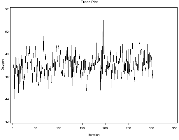
By default, the MI procedure displays solid line segments that connect data points in the trace plot. The plot shows no apparent trends for the variable Oxygen.

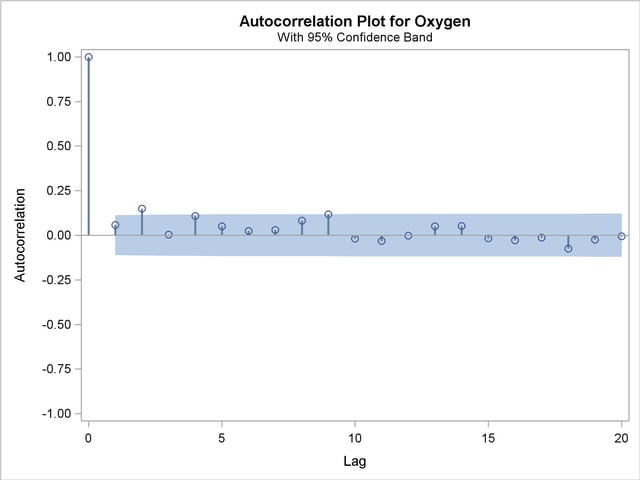
When you use the ACFPLOT(MEAN(OXYGEN)) option, the MI procedure displays an autocorrelation plot for the mean of Oxygen in Output 54.8.2.

Output 54.8.2 Autocorrelation Function Plot for Oxygen

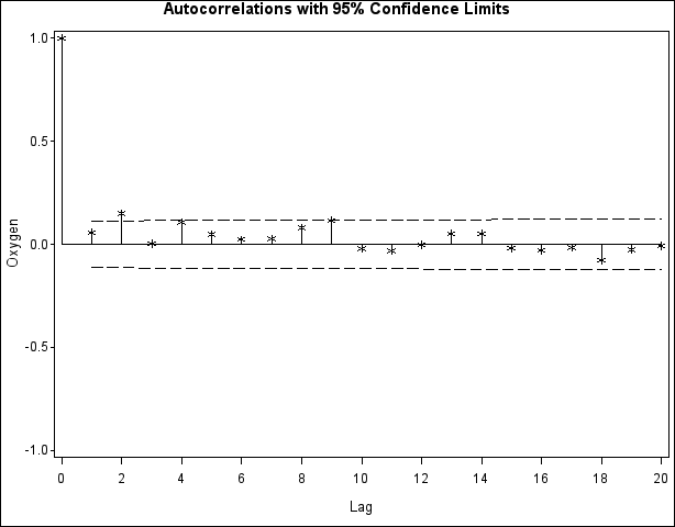
By default, the MI procedure uses the star (*) as the plot symbol to display the points in the plot, a solid line to display the reference line of zero autocorrelation, and a pair of dashed lines to display approximately 95% confidence limits for the autocorrelations. The autocorrelation function plot shows no significant positive or negative autocorrelation.

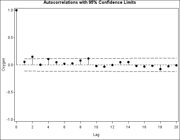
The following statements use display options to modify the autocorrelation function plot for Oxygen in Output 54.8.3:

   proc mi data=FitMiss seed=42037921 noprint nimpute=2;
      mcmc acfplot(mean(Oxygen) / symbol=dot lref=2);
      var Oxygen RunTime RunPulse;
   run;

Output 54.8.3 Autocorrelation Function Plot for Oxygen

You can also create plots for the worst linear function, the means of other variables, the variances of variables, and the covariances between variables. Alternatively, you can use the OUTITER option to save statistics such as the means, standard deviations, covariances, log LR statistic, log LR statistic of the posterior mode, and worst linear function from each iteration in an output data set. Then you can do a more in-depth trace (time series) analysis of the iterations with other procedures, such as PROC AUTOREG and PROC ARIMA in the SAS/ETS User’s Guide.

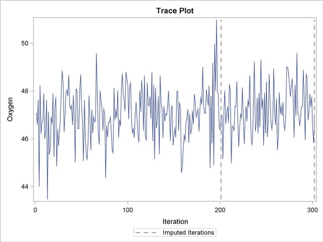
With the ods graphics on statement specified in the following statements, the MI procedure produces the ODS graphs in Output 54.8.4 and Output 54.8.5:

   ods graphics on;
   proc mi data=FitMiss seed=42037921 nimpute=2;
      mcmc plots=(trace(mean(Oxygen)) acf(mean(Oxygen)));
      var Oxygen RunTime RunPulse;
   run;
   ods graphics off;

The TRACE(MEAN(OXYGEN)) option displays the trace plot of means for the variable Oxygen. The dashed vertical lines indicate the imputed iterations—that is, the Oxygen values used in the imputations.

Output 54.8.4 Trace Plot for Oxygen

The ACF(MEAN(OXYGEN)) option displays the autocorrelation plot of means for the variable Oxygen.

Output 54.8.5 Autocorrelation Function Plot for Oxygen

For general information about the ods graphics statement, see Chapter 21, Statistical Graphics Using ODS. For specific information about the graphics available in the MI procedure, see the section ODS Graphics.