| The LOGISTIC Procedure |
| Iterative Algorithms for Model Fitting |
Two iterative maximum likelihood algorithms are available in PROC LOGISTIC. The default is the Fisher scoring method, which is equivalent to fitting by iteratively reweighted least squares. The alternative algorithm is the Newton-Raphson method. Both algorithms give the same parameter estimates; however, the estimated covariance matrix of the parameter estimators can differ slightly. This is due to the fact that Fisher scoring is based on the expected information matrix while the Newton-Raphson method is based on the observed information matrix. In the case of a binary logit model, the observed and expected information matrices are identical, resulting in identical estimated covariance matrices for both algorithms. For a generalized logit model, only the Newton-Raphson technique is available. You can use the TECHNIQUE= option to select a fitting algorithm. Also, the FIRTH option modifies these techniques to perform a bias-reducing penalized maximum likelihood fit.
Iteratively Reweighted Least Squares Algorithm (Fisher Scoring)
Consider the multinomial variable 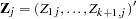 such that
 |
 |
With  denoting the probability that the jth observation has response value i, the expected value of
  is
is  where
where 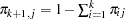 . The covariance matrix of is
  , which is the covariance matrix of a multinomial random variable for one trial with parameter vector
  . Let
. Let  be the vector of regression parameters; in other words,
  . Let
. Let  be the matrix of partial derivatives of with respect to . The estimating equation for the regression parameters is
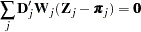 |
where  ,
,  and
and  are the weight and frequency of the
  th observation, and
  is a generalized inverse of
  . PROC LOGISTIC chooses as the inverse of the diagonal matrix with as the diagonal.
With a starting value of  , the maximum likelihood estimate of is obtained iteratively as
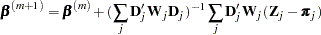 |
where ,  , and are evaluated at
  . The expression after the plus sign is the step size. If the likelihood evaluated at
  is less than that evaluated at , then is recomputed by step-halving or ridging as determined by the value of the RIDGING= option. The iterative scheme continues until convergence is obtained—that is, until is sufficiently close to . Then the maximum likelihood estimate of is
  .
.
The covariance matrix of  is estimated by
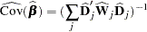 |
where  and
and  are, respectively, and evaluated at .
By default, starting values are zero for the slope parameters, and for the intercept parameters, starting values are the observed cumulative logits (that is, logits of the observed cumulative proportions of response). Alternatively, the starting values can be specified with the INEST= option.
Newton-Raphson Algorithm
For cumulative models, let the parameter vector be 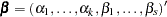 , and for the generalized logit model let
 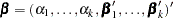 . The gradient vector and the Hessian matrix are given, respectively, by
 |
 |
 |
|||
 |
|
 |
where  is the log likelihood for the th observation. With a starting value of , the maximum likelihood estimate of is obtained iteratively until convergence is obtained:
 |
where  and
and  are evaluated at . If the likelihood evaluated at is less than that evaluated at , then is recomputed by step-halving or ridging.
The covariance matrix of is estimated by
 |
where  is evaluated at .
Firth’s Bias-Reducing Penalized Likelihood
Firth’s method is currently available only for binary logistic models. It replaces the usual score (gradient) equation
 |
where  is the number of parameters in the model, with the modified score equation
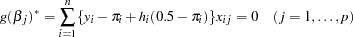 |
where the  s are the
  th diagonal elements of the hat matrix
 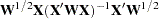 and
and 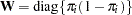 . The Hessian matrix is not modified by this penalty, and the optimization method is performed in the usual manner.
Copyright © 2009 by SAS Institute Inc., Cary, NC, USA. All rights reserved.