| The KRIGE2D Procedure |
| Theoretical Semivariogram Models |
Consider a stochastic spatial process represented by the spatial random field (SRF; see Christakos 1992) {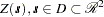 }. PROC VARIOGRAM computes the empirical (also known as sample or experimental) semivariance of
  . Prediction of the spatial process at unsampled locations by techniques such as ordinary kriging requires a theoretical semivariogram or covariance.
When you use PROC VARIOGRAM and PROC KRIGE2D to perform spatial prediction, you must determine a suitable theoretical semivariogram based on the sample semivariogram. There are various methods of fitting semivariogram models, such as least squares, maximum likelihood, and robust methods (Cressie; 1993, Section 2.6). A different approach is manual fitting, where a theoretical semivariogram is chosen based on visual inspection of the empirical estimate; see, for example, Hohn (1988, p. 25).
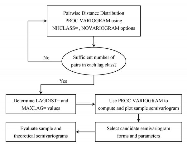
In some cases, a plot of the experimental semivariogram suggests that a single theoretical model is inadequate. Nested models, anisotropic models, and the nugget effect increase the scope of theoretical models available. All of these concepts are discussed in this section. The specification of the final theoretical model is provided by the syntax of PROC KRIGE2D.
Note the general flow of investigation. The empirical semivariogram is computed after a suitable choice is made for the LAGDISTANCE= and MAXLAGS= options in PROC VARIOGRAM, and possibly the NDIR= option or the DIRECTIONS statement for computations in more than one directions. Potential theoretical models (which can also incorporate nesting, anisotropy, and the nugget effect) are then plotted against the empirical semivariogram and evaluated. A suitable theoretical model is found by using the methodology presented in the section Examples: VARIOGRAM Procedure in the VARIOGRAM procedure. The flow of this process is illustrated in Figure 46.5.
Four theoretical models are supported by PROC KRIGE2D: the spherical, Gaussian, exponential, and power models—see also the section Theoretical Semivariogram Models in the VARIOGRAM procedure. For the first three types, the parameters  and
and  , corresponding to the RANGE= and SCALE= options in the MODEL statement in PROC KRIGE2D, have the same dimensions and have similar effects on the shape of
  , as illustrated in the following paragraph.
In particular, the dimension of is the same as the dimension of the variance of the spatial process . The dimension of is length with the same units as  .
.
These four model forms are now examined in more detail.
The Spherical Semivariogram Model
The form of the spherical model is
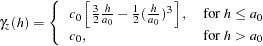 |
The shape is displayed in Figure 46.6, using range  and scale
  .
.
and 
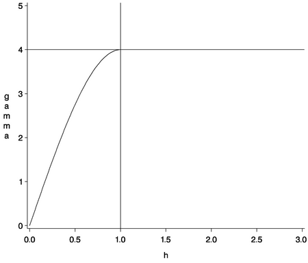
The vertical line at  shows the range of the model.
The horizontal line at 4.0 variance units (corresponding to ) is called the sill. In the case of the spherical model, actually reaches this value. For the following two model types, the sill is a horizontal asymptote.
The Gaussian Semivariogram Model
The form of the Gaussian model is
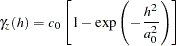 |
The shape is displayed in Figure 46.7, using range and scale .
and
The vertical line at  shows the effective (or practical) range as defined by Deutsch and Journel (1992), or the range
  defined by Christakos (1992). The effective range is the -value where the covariance is approximately 5% of its value at zero.
The horizontal line at 4.0 variance units (corresponding to ) is the sill; approaches the sill asymptotically.
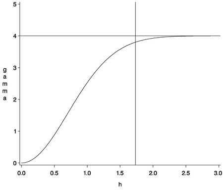
The Exponential Semivariogram Model
The form of the exponential model is
 |
The shape is displayed in Figure 46.8, using range and scale .
and
The vertical line at  is the effective (or practical) range, or the range (that is, the -value where the covariance is approximately 5% of its value at zero).
The horizontal line at 4.0 variance units (corresponding to ) is the sill, as in the previous model types.
It is noted from Figure 46.7 and Figure 46.8 that the major distinguishing feature of the Gaussian and exponential forms is the shape in the neighborhood of the origin  . In general, small lags are important in determining an appropriate theoretical form based on a sample semivariogram.
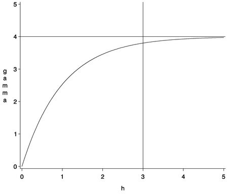
The Power Semivariogram Model
The form of the power model is
 |
For this model, the parameter is a dimensionless quantity, with typical values  . Note that the value of yields a straight line. The parameter has dimensions of the variance, as in the other models. There is no sill for the power model. The shape of the power model with
  and is displayed in Figure 46.9.
and
Nested Models
For a given set of spatial data, a plot of an experimental semivariogram might not seem to fit any of the individual theoretical models. In such a case, you might obtain a more accurate fit if you consider your covariance model to be the sum of two or more covariance structures. Such covariance models are called nested models. Nesting is common in geologic applications where there are correlations at different length scales. At small lag distances , the smaller scale correlations dominate, while the large scale correlations dominate at larger lag distances.
Nested models are permissible covariances if they are the sum of permissible models. Therefore, you can include in a sum any combination of the models presented in the preceding subsections and produce permissible covariance models. As an illustration, consider two semivariogram models: an exponential and a spherical:
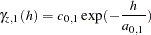 |
and
 |
with  , and
, and  . If both of these correlation structures are present in a spatial process {
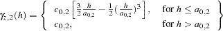
 }, then the semivariance
  of this process can be expressed as
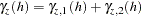 |
In this case, the experimental semivariogram for the process resembles the semivariogram of the sum of  and
and  . This is illustrated in Figure 46.10.
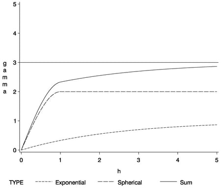
The sum of and in Figure 46.10 does not resemble any single theoretical semivariogram; however, its shape at is similar to a spherical form. The asymptotic approach to a sill at three variance units, along with the shape around , indicates an exponential structure. Note that the sill value  of the sum is the sum of the individual sills
  and
and  . In general, a nested model has a sill equal to the sum of the sills of its nested structures plus the nugget effect, if present.
Refer to Hohn (1988, p. 38ff) for further examples of nested correlation structures.
Copyright © 2009 by SAS Institute Inc., Cary, NC, USA. All rights reserved.