Sparse Storage and Computation

One of the fundamental computational tasks in analyzing a linear mixed model is solving the mixed model equations

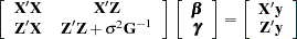where denotes the variance matrix of the random effects. The mixed model crossproduct matrix

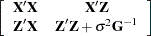is a key component of these equations, and it often has many zero values (George and Liu; 1981). Sparse storage techniques can result in significant savings in both memory and CPU resources. The HPMIXED procedure draws on sparse matrix representation and storage where appropriate or necessary.

Conjugate Gradient Algorithm and Iteration-on-Data Technology

Solving the mixed model equations is a critical component of linear mixed model analysis. The two main components of the preconditioned conjugate gradient (PCCG) algorithm are preconditioning and matrix-vector product computing (Shewchuk; 1994). The algorithm is guaranteed to converge to the solution within iterations, where is equal to the number of distinct eigenvalues of the mixed model equations. This simple yet powerful algorithm can be easily implemented with an iteration-on-data (IOD) technique (Tsuruta, Misztal, and Stranden; 2001) that can yield significant savings of memory resources.

The combination of the PCCG algorithm and iteration on data makes it possible to efficiently compute best linear unbiased predictors (BLUPs) for the random effects in mixed models with large mixed model equations.

Average Information Algorithm

The HPMIXED procedure estimates covariance parameters by restricted maximum likelihood. The default optimization method is a quasi-Newton algorithm. When the Hessian or information matrix is required, the HPMIXED procedure takes advantage of the computational simplifications that are available by averaging information (AI). The AI algorithm (Johnson and Thompson; 1995; Gilmour, Thompson, and Cullis; 1995) replaces the second derivative matrix with the average of the observed and expected information matrices. The computationally intensive trace terms in these information matrices cancel upon averaging. Coarsely, the AI algorithm can be viewed as a hybrid of a Newton-Raphson approach and Fisher scoring.