| The GLMMOD Procedure |
| A One-Way Design |
A one-way analysis of variance considers one treatment factor with two or more treatment levels. This example employs PROC GLMMOD together with PROC REG to perform a one-way analysis of variance to study the effect of bacteria on the nitrogen content of red clover plants. The treatment factor is bacteria strain, and it has six levels. Red clover plants are inoculated with the treatments, and nitrogen content is later measured in milligrams. The data are derived from an experiment by Erdman (1946) and are analyzed in Chapters 7 and 8 of Steel and Torrie (1980). PROC GLMMOD is used to create the design matrix. The following DATA step creates the SAS data set Clover.
      title 'Nitrogen Content of Red Clover Plants';
      data Clover;
         input Strain $ Nitrogen @@;
         datalines;
      3DOK1  19.4 3DOK1  32.6 3DOK1  27.0 3DOK1  32.1 3DOK1  33.0
      3DOK5  17.7 3DOK5  24.8 3DOK5  27.9 3DOK5  25.2 3DOK5  24.3
      3DOK4  17.0 3DOK4  19.4 3DOK4   9.1 3DOK4  11.9 3DOK4  15.8
      3DOK7  20.7 3DOK7  21.0 3DOK7  20.5 3DOK7  18.8 3DOK7  18.6
      3DOK13 14.3 3DOK13 14.4 3DOK13 11.8 3DOK13 11.6 3DOK13 14.2
      COMPOS 17.3 COMPOS 19.4 COMPOS 19.1 COMPOS 16.9 COMPOS 20.8
      ;
The variable Strain contains the treatment levels, and the variable Nitrogen contains the response. The following statements produce the design matrix:
   proc glmmod data=Clover;
      class Strain;
      model Nitrogen = Strain;
   run;
The classification variable, or treatment factor, is specified in the CLASS statement. The MODEL statement defines the response and independent variables. The design matrix produced corresponds to the model
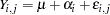 |
where  and
and  .
.
Figure 40.1 and Figure 40.2 display the output produced by these statements. Figure 40.1 displays information about the data set, which is useful for checking your data.
| Class Level Information | ||
|---|---|---|
| Class | Levels | Values |
| Strain | 6 | 3DOK1 3DOK13 3DOK4 3DOK5 3DOK7 COMPOS |
The design matrix, shown in Figure 40.2, consists of seven columns: one for the mean and six for the treatment levels. The vector of responses, Nitrogen, is also displayed.
| Design Points | ||||||||
|---|---|---|---|---|---|---|---|---|
| Observation Number |
Nitrogen | Column Number | ||||||
| 1 | 2 | 3 | 4 | 5 | 6 | 7 | ||
| 1 | 19.4 | 1 | 1 | 0 | 0 | 0 | 0 | 0 |
| 2 | 32.6 | 1 | 1 | 0 | 0 | 0 | 0 | 0 |
| 3 | 27.0 | 1 | 1 | 0 | 0 | 0 | 0 | 0 |
| 4 | 32.1 | 1 | 1 | 0 | 0 | 0 | 0 | 0 |
| 5 | 33.0 | 1 | 1 | 0 | 0 | 0 | 0 | 0 |
| 6 | 17.7 | 1 | 0 | 0 | 0 | 1 | 0 | 0 |
| 7 | 24.8 | 1 | 0 | 0 | 0 | 1 | 0 | 0 |
| 8 | 27.9 | 1 | 0 | 0 | 0 | 1 | 0 | 0 |
| 9 | 25.2 | 1 | 0 | 0 | 0 | 1 | 0 | 0 |
| 10 | 24.3 | 1 | 0 | 0 | 0 | 1 | 0 | 0 |
| 11 | 17.0 | 1 | 0 | 0 | 1 | 0 | 0 | 0 |
| 12 | 19.4 | 1 | 0 | 0 | 1 | 0 | 0 | 0 |
| 13 | 9.1 | 1 | 0 | 0 | 1 | 0 | 0 | 0 |
| 14 | 11.9 | 1 | 0 | 0 | 1 | 0 | 0 | 0 |
| 15 | 15.8 | 1 | 0 | 0 | 1 | 0 | 0 | 0 |
| 16 | 20.7 | 1 | 0 | 0 | 0 | 0 | 1 | 0 |
| 17 | 21.0 | 1 | 0 | 0 | 0 | 0 | 1 | 0 |
| 18 | 20.5 | 1 | 0 | 0 | 0 | 0 | 1 | 0 |
| 19 | 18.8 | 1 | 0 | 0 | 0 | 0 | 1 | 0 |
| 20 | 18.6 | 1 | 0 | 0 | 0 | 0 | 1 | 0 |
| 21 | 14.3 | 1 | 0 | 1 | 0 | 0 | 0 | 0 |
| 22 | 14.4 | 1 | 0 | 1 | 0 | 0 | 0 | 0 |
| 23 | 11.8 | 1 | 0 | 1 | 0 | 0 | 0 | 0 |
| 24 | 11.6 | 1 | 0 | 1 | 0 | 0 | 0 | 0 |
| 25 | 14.2 | 1 | 0 | 1 | 0 | 0 | 0 | 0 |
| 26 | 17.3 | 1 | 0 | 0 | 0 | 0 | 0 | 1 |
| 27 | 19.4 | 1 | 0 | 0 | 0 | 0 | 0 | 1 |
| 28 | 19.1 | 1 | 0 | 0 | 0 | 0 | 0 | 1 |
| 29 | 16.9 | 1 | 0 | 0 | 0 | 0 | 0 | 1 |
| 30 | 20.8 | 1 | 0 | 0 | 0 | 0 | 0 | 1 |
Usually, you will find PROC GLMMOD most useful for the data sets it can create rather than for its displayed output. For example, the following statements use PROC GLMMOD to save the design matrix for the clover study to the data set CloverDesign instead of displaying it.
   proc glmmod data=Clover outdesign=CloverDesign noprint;
      class Strain;
      model Nitrogen = Strain;
   run;
Now you can use the REG procedure to analyze the data, as the following statements demonstrate:
   proc reg data=CloverDesign;
      model Nitrogen = Col2-Col7;
   run;
The results are shown in Figure 40.3.
| Number of Observations Read | 30 |
|---|---|
| Number of Observations Used | 30 |
| Analysis of Variance | |||||
|---|---|---|---|---|---|
| Source | DF | Sum of Squares |
Mean Square |
F Value | Pr > F |
| Model | 5 | 847.04667 | 169.40933 | 14.37 | <.0001 |
| Error | 24 | 282.92800 | 11.78867 | ||
| Corrected Total | 29 | 1129.97467 | |||
| Note: | Model is not full rank. Least-squares solutions for the parameters are not unique. Some statistics will be misleading. A reported DF of 0 or B means that the estimate is biased. |
| Note: | The following parameters have been set to 0, since the variables are a linear combination of other variables as shown. |
| Col7 = | Intercept - Col2 - Col3 - Col4 - Col5 - Col6 |
|---|
| Parameter Estimates | ||||||
|---|---|---|---|---|---|---|
| Variable | Label | DF | Parameter Estimate |
Standard Error |
t Value | Pr > |t| |
| Intercept | Intercept | B | 18.70000 | 1.53549 | 12.18 | <.0001 |
| Col2 | Strain 3DOK1 | B | 10.12000 | 2.17151 | 4.66 | <.0001 |
| Col3 | Strain 3DOK13 | B | -5.44000 | 2.17151 | -2.51 | 0.0194 |
| Col4 | Strain 3DOK4 | B | -4.06000 | 2.17151 | -1.87 | 0.0738 |
| Col5 | Strain 3DOK5 | B | 5.28000 | 2.17151 | 2.43 | 0.0229 |
| Col6 | Strain 3DOK7 | B | 1.22000 | 2.17151 | 0.56 | 0.5794 |
| Col7 | Strain COMPOS | 0 | 0 | . | . | . |
Copyright © 2009 by SAS Institute Inc., Cary, NC, USA. All rights reserved.