Organization of Data for Repeated Measure Analysis

In order to deal efficiently with the correlation of repeated measures, the GLM procedure uses the multivariate method of specifying the model, even if only a univariate analysis is desired. In some cases, data might already be entered in the univariate mode, with each repeated measure listed as a separate observation along with a variable that represents the experimental unit (subject) on which measurement is taken. Consider the following data set Old:

   data Old;
      input Subject Group Time y;
   datalines;
    1 1 1 15
    1 1 2 19
    1 1 3 25
    2 1 1 21
    2 1 2 18
    2 1 3 17
    1 2 1 14
    1 2 2 12
    1 2 3 16
    2 2 1 11
    2 2 2 20
   
   ... more lines ...   

   10 3 1 14
   10 3 2 18
   10 3 3 16
   ;

There are three observations for each subject, corresponding to measurements taken at times 1, 2, and 3. These data could be analyzed using the following statements:

   proc glm data=Old;
      class Group Subject Time;
      model y=Group Subject(Group) Time Group*Time;
      test h=Group e=Subject(Group);
   run;

However, this analysis assumes subjects’ measurements are uncorrelated across time. A repeated measures analysis does not make this assumption. It uses the following data set New:

   data New;
      input Group y1 y2 y3;
   datalines;
   1  15 19 25
   1  21 18 17
   2  14 12 16
   2  11 20 21
   
   ... more lines ...   

   3  14 18 16
   ;

In the data set New, the three measurements for a subject are all in one observation. For example, the measurements for subject 1 for times 1, 2, and 3 are 15, 19, and 25, respectively. For these data, the statements for a repeated measures analysis (assuming default options) are

   proc glm data=New;
      class Group;
      model y1-y3 = Group / nouni;
      repeated Time;
   run;

To convert the univariate form of repeated measures data to the multivariate form, you can use a program like the following:

   proc sort data=Old;
      by Group Subject;
   run;
    
   data New(keep=y1-y3 Group);
      array yy(3)  y1-y3;
      do Time = 1 to 3;
         set Old;
         by Group Subject;
         yy(Time) = y;
         if last.Subject then return;
      end;
   run;

Alternatively, you could use PROC TRANSPOSE to achieve the same results with a program like this one:

   proc sort data=Old;
      by Group Subject;
   run;
    
   proc transpose out=New(rename=(_1=y1 _2=y2 _3=y3));
      by Group Subject;
      id Time;
   run;

See the discussions in SAS Language Reference: Concepts for more information about rearrangement of data sets.

Hypothesis Testing in Repeated Measures Analysis

In repeated measures analysis of variance, the effects of interest are as follows:

• between-subject effects (such as GROUP in the previous example)

• within-subject effects (such as TIME in the previous example)

• interactions between the two types of effects (such as GROUP*TIME in the previous example)

Repeated measures analyses are distinguished from MANOVA because of interest in testing hypotheses about the within-subject effects and the within-subject-by-between-subject interactions.

For tests that involve only between-subjects effects, both the multivariate and univariate approaches give rise to the same tests. These tests are provided for all effects in the MODEL statement, as well as for any CONTRASTs specified. The ANOVA table for these tests is labeled "Tests of Hypotheses for Between Subjects Effects" in the PROC GLM results. These tests are constructed by first adding together the dependent variables in the model. Then an analysis of variance is performed on the sum divided by the square root of the number of dependent variables. For example, the statements

   model y1-y3=group;
   repeated time;

give a one-way analysis of variance that uses 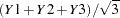as the dependent variable for performing tests of hypothesis on the between-subject effect GROUP. Tests for between-subject effects are equivalent to tests of the hypothesis , where is simply a vector of 1s.

For within-subject effects and for within-subject-by-between-subject interaction effects, the univariate and multivariate approaches yield different tests. These tests are provided for the within-subject effects and for the interactions between these effects and the other effects in the MODEL statement, as well as for any CONTRASTs specified. The univariate tests are displayed in a table labeled "Univariate Tests of Hypotheses for Within Subject Effects." Results for multivariate tests are displayed in a table labeled "Repeated Measures Analysis of Variance."

The multivariate tests provided for within-subjects effects and interactions involving these effects are Wilks’ lambda, Pillai’s trace, Hotelling-Lawley trace, and Roy’s greatest root. For further details on these four statistics, see the "Multivariate Tests" section in Chapter 4, Introduction to Regression Procedures. As an example, the statements

   model y1-y3=group;
   repeated time;

produce multivariate tests for the within-subject effect TIME and the interaction TIME*GROUP.

The multivariate tests for within-subject effects are produced by testing the hypothesis , where the matrix is the usual matrix corresponding to the Type I, Type II, Type III, or Type IV hypotheses test, and the matrix is one of several matrices depending on the transformation that you specify in the REPEATED statement. The only assumption required for valid tests is that the dependent variables in the model have a multivariate normal distribution with a common covariance matrix across the between-subject effects.

The univariate tests for within-subject effects and interactions involving these effects require some assumptions for the probabilities provided by the ordinary tests to be correct. Specifically, these tests require certain patterns of covariance matrices, known as Type H covariances (Huynh and Feldt; 1970). Data with these patterns in the covariance matrices are said to satisfy the Huynh-Feldt condition. You can test this assumption (and the Huynh-Feldt condition) by applying a sphericity test (Anderson; 1958) to any set of variables defined by an orthogonal contrast transformation. Such a set of variables is known as a set of orthogonal components. When you use the PRINTE option in the REPEATED statement, this sphericity test is applied both to the transformed variables defined by the REPEATED statement and to a set of orthogonal components if the specified transformation is not orthogonal. It is the test applied to the orthogonal components that is important in determining whether your data have a Type H covariance structure. When there are only two levels of the within-subject effect, there is only one transformed variable, and a sphericity test is not needed. The sphericity test is labeled "Test for Sphericity" in the output.

If your data satisfy the preceding assumptions, use the usual tests to test univariate hypotheses for the within-subject effects and associated interactions.

If your data do not satisfy the assumption of Type H covariance, an adjustment to numerator and denominator degrees of freedom can be used. Two such adjustments, based on a degrees-of-freedom adjustment factor known as (epsilon) (Box; 1954), are provided in PROC GLM. Both adjustments estimate and then multiply the numerator and denominator degrees of freedom by this estimate before determining significance levels for the tests. Significance levels associated with the adjusted tests are labeled "Adj Pr > F" in the output. The first adjustment, initially proposed for use in data analysis by Greenhouse and Geisser (1959), is labeled "Greenhouse-Geisser Epsilon" and represents the maximum likelihood estimate of Box’s factor. Significance levels associated with adjusted tests are labeled "G-G" in the output. Huynh and Feldt (1976) have shown that the G-G estimate tends to be biased downward (that is, too conservative), especially for small samples, and they have proposed an alternative estimator that is constructed using unbiased estimators of the numerator and denominator of Box’s . Huynh and Feldt’s estimator is labeled "Huynh-Feldt Epsilon" in the PROC GLM output, and the significance levels associated with adjusted tests are labeled "H-F." Although must be in the range of 0 to 1, the H-F estimator can be outside this range. When the H-F estimator is greater than 1, a value of 1 is used in all calculations for probabilities, and the H-F probabilities are not adjusted. In summary, if your data do not meet the assumptions, use adjusted tests. However, when you strongly suspect that your data might not have Type H covariance, all these univariate tests should be interpreted cautiously. In such cases, you should consider using the multivariate tests instead.

The univariate sums of squares for hypotheses involving within-subject effects can be easily calculated from the and matrices corresponding to the multivariate tests described in the section Multivariate Analysis of Variance. If the matrix is orthogonal, the univariate sums of squares is calculated as the trace (sum of diagonal elements) of the appropriate matrix; if it is not orthogonal, PROC GLM calculates the trace of the matrix that results from an orthogonal matrix transformation. The appropriate error term for the univariate tests is constructed in a similar way from the error SSCP matrix and is labeled Error(factorname), where factorname indicates the matrix that is used in the transformation.

When the design specifies more than one repeated measures factor, PROC GLM computes the matrix for a given effect as the direct (Kronecker) product of the matrices defined by the REPEATED statement if the factor is involved in the effect or as a vector of 1s if the factor is not involved. The test for the main effect of a repeated measures factor is constructed using an matrix that corresponds to a test that the mean of the observation is zero. Thus, the main effect test for repeated measures is a test that the means of the variables defined by the matrix are all equal to zero, while interactions involving repeated measures effects are tests that the between-subjects factors involved in the interaction have no effect on the means of the transformed variables defined by the matrix. In addition, you can specify other matrices to test hypotheses of interest by using the CONTRAST statement, since hypotheses defined by CONTRAST statements are also tested in the REPEATED analysis. To see which combinations of the original variables the transformed variables represent, you can specify the PRINTM option in the REPEATED statement. This option displays the transpose of , which is labeled as M in the PROC GLM results. The tests produced are the same for any choice of transformation matrix specified in the REPEATED statement; however, depending on the nature of the repeated measurements being studied, a particular choice of transformation matrix, coupled with the CANONICAL or SUMMARY option, can provide additional insight into the data being studied.

Transformations Used in Repeated Measures Analysis of Variance

As mentioned in the specifications of the REPEATED statement, several different matrices can be generated automatically, based on the transformation that you specify in the REPEATED statement. Remember that both the univariate and multivariate tests that PROC GLM performs are unaffected by the choice of transformation; the choice of transformation is important only when you are trying to study the nature of a repeated measures effect, particularly with the CANONICAL and SUMMARY options. If one of these matrices does not meet your needs for a particular analysis, you might want to use the M= option in the MANOVA statement to perform the tests of interest.

The following sections describe the transformations available in the REPEATED statement, provide an example of the matrix that is produced, and give guidelines for the use of the transformation. As in the PROC GLM output, the displayed matrix is labeled M. This is the matrix.

CONTRAST Transformation

This is the default transformation used by the REPEATED statement. It is useful when one level of the repeated measures effect can be thought of as a control level against which the others are compared. For example, if five drugs are administered to each of several animals and the first drug is a control or placebo, the statements

   proc glm;
      model d1-d5= / nouni;
      repeated drug 5 contrast(1) / summary printm;
   run;

produce the following matrix:

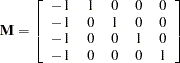When you examine the analysis of variance tables produced by the SUMMARY option, you can tell which of the drugs differed significantly from the placebo.

POLYNOMIAL Transformation

This transformation is useful when the levels of the repeated measure represent quantitative values of a treatment, such as dose or time. If the levels are unequally spaced, level values can be specified in parentheses after the number of levels in the REPEATED statement. For example, if five levels of a drug corresponding to 1, 2, 5, 10, and 20 milligrams are administered to different treatment groups, represented by the variable group, the statements

   proc glm;
      class group;
      model r1-r5=group / nouni;
      repeated dose 5 (1 2 5 10 20) polynomial / summary printm;
   run;
    

produce the following matrix:

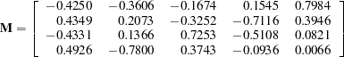The SUMMARY option in this example provides univariate ANOVAs for the variables defined by the rows of this matrix. In this case, they represent the linear, quadratic, cubic, and quartic trends for dose and are labeled dose_1, dose_2, dose_3, and dose_4, respectively.

HELMERT Transformation

Since the Helmert transformation compares a level of a repeated measure to the mean of subsequent levels, it is useful when interest lies in the point at which responses cease to change. For example, if four levels of a repeated measures factor represent responses to treatments administered over time to males and females, the statements

   proc glm;
      class sex;
      model resp1-resp4=sex / nouni;
      repeated trtmnt 4 helmert / canon printm;
   run;

produce the following matrix:

MEAN Transformation

This transformation can be useful in the same types of situations in which the CONTRAST transformation is useful. If you substitute the following statement for the REPEATED statement shown in the CONTRAST Transformation section,

   repeated drug 5 mean / printm;

the following matrix is produced:

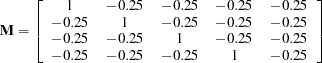As with the CONTRAST transformation, if you want to omit a level other than the last, you can specify it in parentheses after the keyword MEAN in the REPEATED statement.

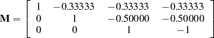
PROFILE Transformation

When a repeated measure represents a series of factors administered over time, but a polynomial response is unreasonable, a profile transformation might prove useful. As an example, consider a training program in which four different methods are employed to teach students at several different schools. The repeated measure is the score on tests administered after each of the methods is completed. The statements

   proc glm;
      class school;
      model t1-t4=school / nouni;
      repeated method 4 profile / summary nom printm;
   run;

produce the following matrix:

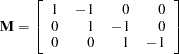To determine the point at which an improvement in test scores takes place, you can examine the analyses of variance for the transformed variables representing the differences between adjacent tests. These analyses are requested by the SUMMARY option in the REPEATED statement, and the variables are labeled METHOD.1, METHOD.2, and METHOD.3.