| The GLIMMIX Procedure |
Example 38.6 Radial Smoothing of Repeated Measures Data
This example of a repeated measures study is taken from Diggle, Liang, and Zeger (1994, p. 100). The data consist of body weights of 27 cows, measured at 23 unequally spaced time points over a period of approximately 22 months. Following Diggle, Liang, and Zeger (1994), one animal is removed from the analysis, one observation is removed according to their Figure 5.7, and the time is shifted to start at 0 and is measured in 10-day increments. The design is a  factorial, and the factors are the infection of an animal with M. paratuberculosis and whether the animal is receiving iron dosing.
The following DATA steps create the data and arrange them in univariate format.
   data times;
     input time1-time23;
     datalines;
    122  150  166  179  219  247  276  296  324  354  380  445
    478  508  536  569  599  627  655  668  723  751  781
   ;

   data cows;
     if _n_ = 1 then merge times;
     array t{23} time1   - time23;
     array w{23} weight1 - weight23;
     input cow iron infection weight1-weight23 @@;
     do i=1 to 23;
        weight = w{i};
        tpoint = (t{i}-t{1})/10;
        output;
     end;
     keep cow iron infection tpoint weight;
     datalines;
     1 0 0  4.7    4.905  5.011  5.075  5.136  5.165  5.298  5.323
            5.416  5.438  5.541  5.652  5.687  5.737  5.814  5.799
            5.784  5.844  5.886  5.914  5.979  5.927  5.94
     2 0 0  4.868  5.075  5.193  5.22   5.298  5.416  5.481  5.521
            5.617  5.635  5.687  5.768  5.799  5.872  5.886  5.872
            5.914  5.966  5.991  6.016  6.087  6.098  6.153
     3 0 0  4.868  5.011  5.136  5.193  5.273  5.323  5.416  5.46
            5.521  5.58   5.617  5.687  5.72   5.753  5.784  5.784
            5.784  5.814  5.829  5.872  5.927  5.9    5.991
     4 0 0  4.828  5.011  5.136  5.193  5.273  5.347  5.438  5.561
            5.541  5.598  5.67    .     5.737  5.844  5.858  5.872
            5.886  5.927  5.94   5.979  6.052  6.028  6.12
     5 1 0  4.787  4.977  5.043  5.136  5.106  5.298  5.298  5.371
            5.438  5.501  5.561  5.652  5.67   5.737  5.784  5.768
            5.784  5.784  5.829  5.858  5.914  5.9    5.94
     6 1 0  4.745  4.868  5.043  5.106  5.22   5.298  5.347  5.347
            5.416  5.501  5.561  5.58   5.687  5.72   5.737  5.72
            5.737  5.753  5.768  5.784  5.844  5.844  5.9
     7 1 0  4.745  4.905  5.011  5.106  5.165  5.273  5.371  5.416
            5.416  5.521  5.541  5.635  5.687  5.704  5.784  5.768
            5.768  5.814  5.829  5.858  5.94   5.94   6.004
     8 0 1  4.942  5.106  5.136  5.193  5.298  5.347  5.46   5.521
            5.561  5.58   5.635  5.704  5.784  5.823  5.858  5.9
            5.94   5.991  6.016  6.064  6.052  6.016  5.979
     9 0 1  4.605  4.745  4.868  4.905  4.977  5.22   5.165  5.22
            5.22   5.247  5.298  5.416  5.501  5.521  5.58   5.58
            5.635  5.67   5.72   5.753  5.799  5.829  5.858
    10 0 1  4.7    4.868  4.905  4.977  5.011  5.106  5.165  5.22
            5.22   5.22   5.273  5.384  5.438  5.438  5.501  5.501
            5.541  5.598  5.58   5.635  5.687  5.72   5.704
    11 0 1  4.828  5.011  5.075  5.165  5.247  5.323  5.394  5.46
            5.46   5.501  5.541  5.609  5.687  5.704  5.72   5.704
            5.704  5.72   5.737  5.768  5.858  5.9    5.94
    12 0 1  4.7    4.828  4.905  5.011  5.075  5.165  5.247  5.298
            5.298  5.323  5.416  5.505  5.561  5.58   5.561  5.635
            5.687  5.72   5.72   5.737  5.784  5.814  5.799
    13 0 1  4.828  5.011  5.075  5.136  5.22   5.273  5.347  5.416
            5.438  5.416  5.521  5.628  5.67   5.687  5.72   5.72
            5.799  5.858  5.872  5.914  5.94   5.991  6.016
    14 0 1  4.828  4.942  5.011  5.075  5.075  5.22   5.273  5.298
            5.323  5.298  5.394  5.489  5.541  5.58   5.617  5.67
            5.704  5.753  5.768  5.814  5.872  5.927  5.927
    15 0 1  4.745  4.905  4.977  5.075  5.193  5.22   5.298  5.323
            5.394  5.394  5.438  5.583  5.617  5.652  5.687  5.72
            5.753  5.768  5.814  5.844  5.886  5.886  5.886
    16 0 1  4.7    4.868  5.011  5.043  5.106  5.165  5.247  5.298
            5.347  5.371  5.438  5.455  5.617  5.635  5.704  5.737
            5.784  5.768  5.814  5.844  5.886  5.94   5.927
    17 1 1  4.605  4.787  4.828  4.942  5.011  5.136  5.22   5.247
            5.273  5.247  5.347  5.366  5.416  5.46   5.541  5.481
            5.501  5.635  5.652  5.598  5.635  5.635  5.598
    18 1 1  4.828  4.977  5.011  5.136  5.273  5.298  5.371  5.46
            5.416  5.416  5.438  5.557  5.617  5.67   5.72   5.72
            5.799  5.858  5.886  5.914  5.979  6.004  6.028
    19 1 1  4.7    4.905  4.942  5.011  5.043  5.136  5.193  5.193
            5.247  5.22   5.323  5.338  5.371  5.394  5.438  5.416
            5.501  5.561  5.541  5.58   5.652  5.67   5.704
    20 1 1  4.745  4.905  4.977  5.043  5.136  5.273  5.347  5.394
            5.416  5.394  5.521  5.617  5.617  5.617  5.67   5.635
            5.652  5.687  5.652  5.617  5.687  5.768  5.814
    21 1 1  4.787  4.942  4.977  5.106  5.165  5.247  5.323  5.416
            5.394  5.371  5.438  5.521  5.521  5.561  5.635  5.617
            5.687  5.72   5.737  5.737  5.768  5.768  5.704
    22 1 1  4.605  4.828  4.828  4.977  5.043  5.165  5.22   5.273
            5.247  5.22   5.298  5.375  5.371  5.416  5.501  5.501
            5.521  5.561  5.617  5.635  5.72   5.737  5.768
    23 1 1  4.7    4.905  5.011  5.075  5.106  5.22   5.22   5.298
            5.323  5.347  5.416  5.472  5.501  5.541  5.598  5.598
            5.598  5.652  5.67   5.704  5.737  5.768  5.784
    24 1 1  4.745  4.942  5.011  5.075  5.106  5.247  5.273  5.323
            5.347  5.371  5.416  5.481  5.501  5.541  5.598  5.598
            5.635  5.687  5.704  5.72   5.829  5.844  5.9
    25 1 1  4.654  4.828  4.828  4.977  4.977  5.043  5.136  5.165
            5.165  5.165  5.193  5.204  5.22   5.273  5.371  5.347
            5.46   5.58   5.635  5.67   5.753  5.799  5.844
    26 1 1  4.828  4.977  5.011  5.106  5.165  5.22   5.273  5.323
            5.371  5.394  5.46   5.576  5.652  5.617  5.687  5.67
            5.72   5.784  5.784  5.784  5.829  5.814  5.844
   ;
The mean response profiles of the cows are not of particular interest; what matters are inferences about the Iron effect, the Infection effect, and their interaction. Nevertheless, the body weight of the cows changes over the 22-month period, and you need to account for these changes in the analysis. A reasonable approach is to apply the approximate low-rank smoother to capture the trends over time. This approach frees you from having to stipulate a parametric model for the response trajectories over time. In addition, you can test hypotheses about the smoothing parameter; for example, whether it should be varied by treatment.
The following statements fit a model with a factorial treatment structure and smooth trends over time, choosing the Newton-Raphson algorithm with ridging for the optimization:
   proc glimmix data=cows;
     t2 = tpoint / 100;
     class cow iron infection;
     model weight = iron infection iron*infection tpoint;
     random t2 / type=rsmooth subject=cow
                      knotmethod=kdtree(bucket=100 knotinfo);
     output out=gmxout pred(blup)=pred;
     nloptions tech=newrap;
   run;
The continuous time effect appears in both the MODEL statement (tpoint) and the RANDOM statement (t2). Because the variance of the radial smoothing component depends on the temporal metric, the time scale was rescaled for the RANDOM effect to move the parameter estimate away from the boundary. The knots of the radial smoother are selected as the vertices of a k-d tree. Specifying BUCKET=100 sets the bucket size of the tree to  . Because measurements at each time point are available for 26 (or 25) cows, this groups approximately four time points in a single bucket. The KNOTINFO keyword of the KNOTMETHOD= option requests a printout of the knot locations for the radial smoother. The OUTPUT statement saves the predictions of the mean of each observations to the data set gmxout. Finally, the TECH=NEWRAP option in the NLOPTIONS statement specifies the Newton-Raphson algorithm for the optimization technique.
The "Class Level Information" table lists the number of levels of the Cow, Iron, and Infection effects (Output 38.6.1).
| Model Information | |
|---|---|
| Data Set | WORK.COWS |
| Response Variable | weight |
| Response Distribution | Gaussian |
| Link Function | Identity |
| Variance Function | Default |
| Variance Matrix Blocked By | cow |
| Estimation Technique | Restricted Maximum Likelihood |
| Degrees of Freedom Method | Containment |
The "Radial Smoother Knots for RSmooth(t2)" table displays the knots computed from the vertices of the t2 k-d tree (Output 38.6.2). Notice that knots are spaced unequally and that the extreme time points are among the knot locations. The "Number of Observations" table shows that one observation was not used in the analysis. The 12th observation for cow 4 has a missing value.
The "Dimensions" table shows that the model contains only two covariance parameters, the G-side variance of the spline coefficients ( ) and the R-side scale parameter (
 , Output 38.6.3). For each subject (cow), there are nine columns in the
  matrix, one per knot location. The GLIMMIX procedure processes these data by subjects (cows).
The "Optimization Information" table displays information about the optimization process. Because fixed effects and the residual scale parameter can be profiled from the optimization, the iterative algorithm involves only a single covariance parameter, the variance of the spline coefficients (Output 38.6.4).
After 11 iterations, the optimization process terminates (Output 38.6.5). In this case, the absolute gradient convergence criterion was met.
| Iteration History | |||||
|---|---|---|---|---|---|
| Iteration | Restarts | Evaluations | Objective Function |
Change | Max Gradient |
| 0 | 0 | 4 | -1302.549272 | . | 20.33682 |
| 1 | 0 | 3 | -1451.587367 | 149.03809501 | 9.940495 |
| 2 | 0 | 3 | -1585.640946 | 134.05357887 | 4.71531 |
| 3 | 0 | 3 | -1694.516203 | 108.87525722 | 2.176741 |
| 4 | 0 | 3 | -1775.290458 | 80.77425512 | 0.978577 |
| 5 | 0 | 3 | -1829.966584 | 54.67612585 | 0.425724 |
| 6 | 0 | 3 | -1862.878184 | 32.91160012 | 0.175992 |
| 7 | 0 | 3 | -1879.329133 | 16.45094875 | 0.066061 |
| 8 | 0 | 3 | -1885.175082 | 5.84594887 | 0.020137 |
| 9 | 0 | 3 | -1886.238032 | 1.06295071 | 0.00372 |
| 10 | 0 | 3 | -1886.288519 | 0.05048659 | 0.000198 |
| 11 | 0 | 3 | -1886.288673 | 0.00015425 | 6.364E-7 |
The generalized chi-square statistic in the "Fit Statistics" table is small for this model (Output 38.6.6). There is very little residual variation. The radial smoother is associated with 433.55 residual degrees of freedom, computed as 597 minus the trace of the smoother matrix.
| Fit Statistics | |
|---|---|
| -2 Res Log Likelihood | -1886.29 |
| AIC (smaller is better) | -1882.29 |
| AICC (smaller is better) | -1882.27 |
| BIC (smaller is better) | -1879.77 |
| CAIC (smaller is better) | -1877.77 |
| HQIC (smaller is better) | -1881.56 |
| Generalized Chi-Square | 0.47 |
| Gener. Chi-Square / DF | 0.00 |
| Radial Smoother df(res) | 433.55 |
The "Covariance Parameter Estimates" table in Output 38.6.7 displays the estimates of the covariance parameters. The variance of the random spline coefficients is estimated as  , and the scale parameter (=residual variance) estimate is
  = 0.0008.
The "Type III Tests of Fixed Effects" table displays  tests for the fixed effects in the MODEL statement (Output 38.6.8). There is a strong infection effect as well as the absence of an interaction between infection with M. paratuberculosis and iron dosing. It is important to note, however, that the interpretation of these tests rests on the assumption that the random effects in the mixed model have zero mean; in this case, the radial smoother coefficients.
A graph of the observed data and fitted profiles in the four groups is produced with the following statements (Output 38.6.9):
   data plot; set gmxout;
     length group $26;
          if (iron=0) and (infection=0) then group='Control Group (n=4)';
     else if (iron=1) and (infection=0) then group='Iron - No Infection (n=3)';
     else if (iron=0) and (infection=1) then group='No Iron - Infection (n=9)';
     else group = 'Iron - Infection (n=10)';
   run;
   proc sort data=plot; by group cow;
   run;

   proc sgpanel data=plot noautolegend;
     title 'Radial Smoothing With Cow-Specific Trends';
     label tpoint='Time' weight='log(Weight)';
     panelby group / columns=2 rows=2;
     scatter x=tpoint y=weight;
     series  x=tpoint y=pred / group=cow lineattrs=GraphFit;
   run;
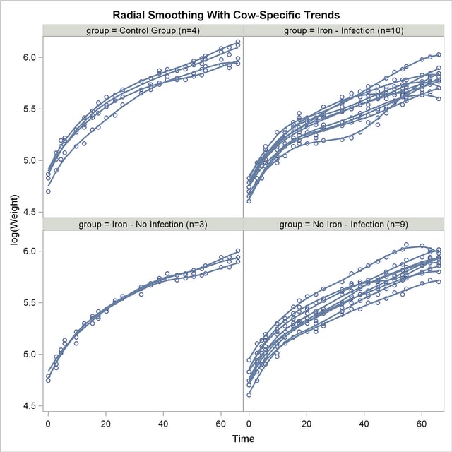
The trends are quite smooth, and you can see how the radial smoother adapts to the cow-specific profile. This is the reason for the small scale parameter estimate,  . Comparing the panels at the top to the panels at the bottom of Output 38.6.9 reveals the effect of Infection. A comparison of the panels on the left to those on the right indicates the weak Iron effect.
The smoothing parameter in this analysis is related to the covariance parameter estimates. Because there is only one radial smoothing variance component, the amount of smoothing is the same in all four treatment groups. To test whether the smoothing parameter should be varied by group, you can refine the analysis of the previous model. The following statements fit the same general model, but they vary the covariance parameters by the levels of the Iron*Infection interaction. This is accomplished with the GROUP= option in the RANDOM statement.
   ods select OptInfo FitStatistics CovParms;
   proc glimmix data=cows;
     t2 = tpoint / 100;
     class cow iron infection;
     model weight = iron infection iron*infection tpoint;
     random t2 / type=rsmooth
                 subject=cow
                 group=iron*infection
                 knotmethod=kdtree(bucket=100);
     nloptions tech=newrap;
   run;
All observations that have the same value combination of the Iron and Infection effects share the same covariance parameter. As a consequence, you obtain different smoothing parameters result in the four groups.
In Output 38.6.10, the "Optimization Information" table shows that there are now four covariance parameters in the optimization, one spline coefficient variance for each group.
| Optimization Information | |
|---|---|
| Optimization Technique | Newton-Raphson |
| Parameters in Optimization | 4 |
| Lower Boundaries | 4 |
| Upper Boundaries | 0 |
| Fixed Effects | Profiled |
| Residual Variance | Profiled |
| Starting From | Data |
| Fit Statistics | |
|---|---|
| -2 Res Log Likelihood | -1887.95 |
| AIC (smaller is better) | -1877.95 |
| AICC (smaller is better) | -1877.85 |
| BIC (smaller is better) | -1871.66 |
| CAIC (smaller is better) | -1866.66 |
| HQIC (smaller is better) | -1876.14 |
| Generalized Chi-Square | 0.48 |
| Gener. Chi-Square / DF | 0.00 |
| Radial Smoother df(res) | 434.72 |
| Covariance Parameter Estimates | ||||
|---|---|---|---|---|
| Cov Parm | Subject | Group | Estimate | Standard Error |
| Var[RSmooth(t2)] | cow | iron*infection 0 0 | 0.4788 | 0.1922 |
| Var[RSmooth(t2)] | cow | iron*infection 0 1 | 0.5152 | 0.1182 |
| Var[RSmooth(t2)] | cow | iron*infection 1 0 | 0.4904 | 0.2195 |
| Var[RSmooth(t2)] | cow | iron*infection 1 1 | 0.7105 | 0.1409 |
| Residual | 0.000807 | 0.000060 | ||
Varying this variance component by groups has changed the  2 Res Log Likelihood from
  to
to  (Output 38.6.10). The difference,
  , can be viewed (asymptotically) as the realization of a chi-square random variable with three degrees of freedom. The difference is not significant (
 ). The "Covariance Parameter Estimates" table confirms that the estimates of the spline coefficient variance are quite similar in the four groups, ranging from
  to
to  .
.
Finally, you can apply a different technique for varying the temporal trends among the cows. From Output 38.6.9 it appears that an assumption of parallel trends within groups might be reasonable. In other words, you can fit a model in which the "overall" trend over time in each group is modeled nonparametrically, and this trend is shifted up or down to capture the behavior of the individual cow. You can accomplish this with the following statements:
   ods select FitStatistics CovParms;
   proc glimmix data=cows;
      t2 = tpoint / 100;
      class cow iron infection;
      model weight = iron infection iron*infection tpoint;
      random t2 / type=rsmooth
                  subject=iron*infection
                  knotmethod=kdtree(bucket=100);
      random intercept / subject=cow;
      output out=gmxout pred(blup)=pred;
      nloptions tech=newrap;
   run;
There are now two subject effects in this analysis. The first RANDOM statement applies the radial smoothing and identifies the experimental conditions as the subject. For each condition, a separate realization of the random spline coefficients is obtained. The second RANDOM statement adds a random intercept to the trend for each cow. This random intercept results in the parallel shift of the trends over time.
Results from this analysis are shown in Output 38.6.11.
| Fit Statistics | |
|---|---|
| -2 Res Log Likelihood | -1788.52 |
| AIC (smaller is better) | -1782.52 |
| AICC (smaller is better) | -1782.48 |
| BIC (smaller is better) | -1788.52 |
| CAIC (smaller is better) | -1785.52 |
| HQIC (smaller is better) | -1788.52 |
| Generalized Chi-Square | 1.17 |
| Gener. Chi-Square / DF | 0.00 |
| Radial Smoother df(res) | 547.21 |
| Covariance Parameter Estimates | |||
|---|---|---|---|
| Cov Parm | Subject | Estimate | Standard Error |
| Var[RSmooth(t2)] | iron*infection | 0.5398 | 0.1940 |
| Intercept | cow | 0.007122 | 0.002173 |
| Residual | 0.001976 | 0.000121 | |
Because the parallel shift model is not nested within either one of the previous models, the models cannot be compared with a likelihood ratio test. However, you can draw on the other fit statistics.
All statistics indicate that this model does not fit the data as well as the initial model that varies the spline coefficients by cow. The Pearson chi-square statistic is more than twice as large as in the previous model, indicating much more residual variation in the fit. On the other hand, this model generates only four sets of spline coefficients, one for each treatment group, and thus retains more residual degrees of freedom.
The "Covariance Parameter Estimates" table in Output 38.6.11 displays the solutions for the covariance parameters. The estimate of the variance of the spline coefficients is not that different from the estimate obtained in the first model ( ). The residual variance, however, has more than doubled.
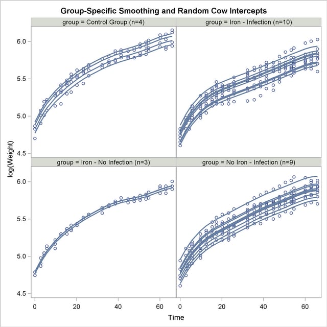
Using similar SAS statements as previously, you can produce a plot of the observed and predicted profiles (Output 38.6.12).
The parallel shifts of the nonparametric smooths are clearly visible in Output 38.6.12. In the groups receiving only iron or only an infection, the parallel lines assumption holds quite well. In the control group and the group receiving iron and the infection, the parallel shift assumption does not hold as well. Two of the profiles in the iron-only group are nearly indistinguishable.
This example demonstrates that mixed model smoothing techniques can be applied not only to achieve scatter plot smoothing, but also to longitudinal or repeated measures data. You can then use the SUBJECT= option in the RANDOM statement to obtain independent sets of spline coefficients for different subjects, and the GROUP= option in the RANDOM statement to vary the degree of smoothing across groups. Also, radial smoothers can be combined with other random effects. For the data considered here, the appropriate model is one with a single smoothing parameter for all treatment group and cow-specific spline coefficients.
Copyright © 2009 by SAS Institute Inc., Cary, NC, USA. All rights reserved.