Profile Likelihood Bounds

The likelihood ratio test statistic for testing is

where is the likelihood estimate of under the restriction that . To invert this test, a function is defined that returns the maximum likelihood for a fixed value of by seeking the maximum over the remaining parameters. This function is termed the profile likelihood (Pawitan 2001, Ch. 3.4),

In computing , is fixed at and is estimated. In mixed models, this step typically requires a separate, iterative optimization to find the estimate of while is held fixed. The profile likelihood confidence interval for is then defined as the set of values for that satisfy

The GLIMMIX procedure seeks the values and that mark the endpoints of the set around that satisfy the inequality. The values and are then called the confidence bounds for . Note that the GLIMMIX procedure assumes that the confidence region is not disjoint and relies on the convexity of .

It is not always possible to find values and that satisfy the inequalities. For example, when the parameter space is ( and

a lower bound cannot be found at the desired confidence level. The GLIMMIX procedure reports the right-tail probabilities that are achieved by the underlying likelihood ratio statistic separately for lower and upper bounds.

Effect of Scale Parameter

When a scale parameter is eliminated from the optimization by profiling from the likelihood, some parameters might be expressed as ratios with in the optimization. This is the case, for example, in variance component models. The profile likelihood confidence bounds are reported on the scale of the parameter in the overall optimization. In case parameters are expressed as ratios with or functions of , the column RatioEstimate is added to the "Covariance Parameter Estimates" table. If parameters are expressed as ratios with and you want confidence bounds for the unscaled parameter, you can prevent profiling of from the optimization with the NOPROFILE option in the PROC GLIMMIX statement, or choose estimated likelihood confidence bounds with the TYPE=ELR suboption of the CL option in the COVTEST statement. Note that the NOPROFILE option is automatically in effect with METHOD=LAPLACE and METHOD=QUAD.

Estimated Likelihood Bounds

Computing profile likelihood ratio confidence bounds can be computationally expensive, because of the need to repeatedly estimate in a constrained optimization. A computationally simpler method to construct confidence bounds from likelihood-based quantities is to use the estimated likelihood (Pawitan 2001, Ch. 10.7) instead of the profile likelihood. An estimated likelihood technique replaces the nuisance parameters in the test inversion with some other estimate. If you choose the TYPE=ELR suboption of the CL option in the COVTEST statement, the GLIMMIX procedure holds the nuisance parameters fixed at the likelihood estimates. The estimated likelihood statistic for inversion is then

where are the elements of that correspond to the nuisance parameters. As the values of are varied, no reestimation of takes place. Although computationally more economical, estimated likelihood intervals do not take into account the variability associated with the nuisance parameters. Their coverage can be satisfactory if the parameter of interest is not (or only weakly) correlated with the nuisance parameters. Estimated likelihood ratio intervals can fall short of the nominal coverage otherwise.

Figure 38.11 depicts profile and estimated likelihood ratio intervals for the parameter in a two-parameter compound-symmetric model, , in which the correlation between the covariance parameters is small. The elliptical shape traces the set of values for which the likelihood ratio test rejects the hypothesis of equality with the solution. The interior of the ellipse is the "acceptance" region of the test. The solid and dashed lines depict the PLR and ELR confidence limits for , respectively. Note that both confidence limits intersect the ellipse and that the ELR interval passes through the REML estimate of . The PLR bounds are found as those points intersecting the ellipse, where equals the constrained REML estimate.

Figure 38.11 PLR and ELR Intervals, Small Correlation between Parameters

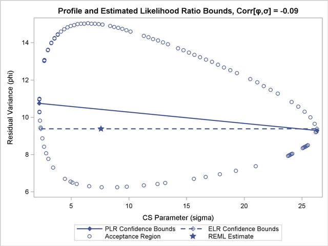
The major axes of the ellipse in Figure 38.11 are nearly aligned with the major axes of the coordinate system. As a consequence, the line connecting the PLR bounds passes close to the REML estimate in the full model. As a result, ELR bounds will be similar to PLR bounds. Figure 38.12 displays a different scenario, a two-parameter AR(1) covariance structure with a more substantial correlation between the AR(1) parameter () and the residual variance ().

Figure 38.12 PLR and ELR Intervals, Large Correlation between Parameters

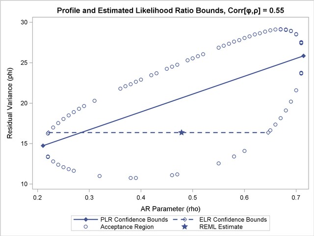
The correlation between the parameters yields an acceptance region whose major axes are not aligned with the axes of the coordinate system. The ELR bound for passes through the REML estimate of from the full model and is much shorter than the PLR interval. The PLR interval aligns with the major axis of the acceptance region; it is the preferred confidence interval.