| The FACTOR Procedure |
Example 33.2 Principal Factor Analysis
This example uses the data presented in Example 33.1, and performs a principal factor analysis with squared multiple correlations for the prior communality estimates (PRIORS=SMC). Unlike Example 33.1, which analyzes the principal components, the current analysis is based on a common factor model.
To help determine whether the common factor model is appropriate, Kaiser’s measure of sampling adequacy (MSA) is requested, and the residual correlations and partial correlations are computed (RESIDUAL).
The ROTATE= and REORDER options are specified to enhance factor interpretability. The ROTATE=PROMAX option produces an orthogonal varimax prerotation (default) followed by an oblique Procrustes rotation, and the REORDER option reorders the variables according to their largest factor loadings. An OUTSTAT= data set is created by PROC FACTOR and displayed in Output 33.2.12.
PROC FACTOR can produce high-quality graphs that are very useful to interpret the factor solutions. To request these graphs, you must first enable ODS Graphics by specifying the ods graphics on statement, as shown in the following code. All ODS graphs in PROC FACTOR are requested with the PLOTS= option. In this example, a scree plot is requested to help you determine the number of factors. Loading plots for the initial unrotated solution, prerotated (varimax) solution, and promax-rotated solution are also requested to help you visualize the patterns of factor loadings in various stages.
   ods graphics on;

   title3 'Principal Factor Analysis with Promax Rotation';
   proc factor data=SocioEconomics
      priors=smc msa residual
      rotate=promax reorder
      outstat=fact_all
      plots=(scree initloadings preloadings loadings);
   run;

   ods graphics off;
Output 33.2.1 displays the results of the principal factor extraction.
| Partial Correlations Controlling all other Variables | |||||
|---|---|---|---|---|---|
| Population | School | Employment | Services | HouseValue | |
| Population | 1.00000 | -0.54465 | 0.97083 | 0.09612 | 0.15871 |
| School | -0.54465 | 1.00000 | 0.54373 | 0.04996 | 0.64717 |
| Employment | 0.97083 | 0.54373 | 1.00000 | 0.06689 | -0.25572 |
| Services | 0.09612 | 0.04996 | 0.06689 | 1.00000 | 0.59415 |
| HouseValue | 0.15871 | 0.64717 | -0.25572 | 0.59415 | 1.00000 |
| Kaiser's Measure of Sampling Adequacy: Overall MSA = 0.57536759 | ||||
|---|---|---|---|---|
| Population | School | Employment | Services | HouseValue |
| 0.47207897 | 0.55158839 | 0.48851137 | 0.80664365 | 0.61281377 |
| Prior Communality Estimates: SMC | ||||
|---|---|---|---|---|
| Population | School | Employment | Services | HouseValue |
| 0.96859160 | 0.82228514 | 0.96918082 | 0.78572440 | 0.84701921 |
| Eigenvalues of the Reduced Correlation Matrix: Total = 4.39280116 Average = 0.87856023 | ||||
|---|---|---|---|---|
| Eigenvalue | Difference | Proportion | Cumulative | |
| 1 | 2.73430084 | 1.01823217 | 0.6225 | 0.6225 |
| 2 | 1.71606867 | 1.67650586 | 0.3907 | 1.0131 |
| 3 | 0.03956281 | 0.06408626 | 0.0090 | 1.0221 |
| 4 | -.02452345 | 0.04808427 | -0.0056 | 1.0165 |
| 5 | -.07260772 | -0.0165 | 1.0000 | |
If the data are appropriate for the common factor model, the partial correlations controlling the other variables should be small compared to the original correlations. The partial correlation between the variables School and HouseValue, for example, is  , slightly less than the original correlation of
  . The partial correlation between Population and School is
  , which is much larger in absolute value than the original correlation; this is an indication of trouble. Kaiser’s MSA is a summary, for each variable and for all variables together, of how much smaller the partial correlations are than the original correlations. Values of
  or
or  are considered good, while MSAs below
  are unacceptable. The variables Population, School, and Employment have very poor MSAs. Only the Services variable has a good MSA. The overall MSA of
  is sufficiently poor that additional variables should be included in the analysis to better define the common factors. A commonly used rule is that there should be at least three variables per factor. In the following analysis, there seems to be two common factors in these data, so more variables are needed for a reliable analysis.
The SMCs are all fairly large; hence, the factor loadings do not differ greatly from those in the principal component analysis.
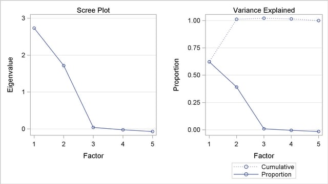
The eigenvalues in Output 33.2.1 show clearly that two common factors are present. The first two largest positive eigenvalues account for  of the common variance. This is possible because the reduced correlation matrix, in general, is not necessarily positive definite, and negative eigenvalues for the matrix are possible. These cumulative proportions of common variance explained by factors are plotted in the right panel of Output 33.2.2, which shows that the curve flattens out essentially after the second factor. Showing in the left panel of Output 33.2.2 is the scree plot, which displays a sharp bend at the third eigenvalue, reinforcing the conclusion that two common factors are present.
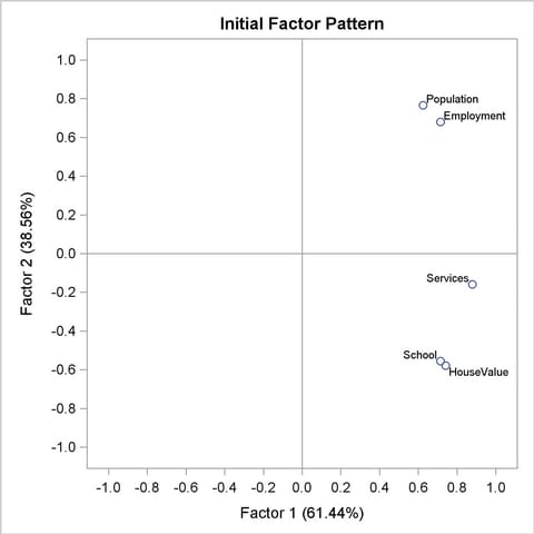
As displayed in Output 33.2.3, the principal factor pattern is similar to the principal component pattern seen in Example 33.1. For example, the variable Services has the largest loading on the first factor, and the Population variable has the smallest. The variables Population and Employment have large positive loadings on the second factor, and the HouseValue and School variables have large negative loadings.
The final communality estimates are all fairly close to the priors. Only the communality for the variable HouseValue increased appreciably, from 0.847 to 0.885. Nearly 100% of the common variance is accounted for. The residual correlations (off-diagonal elements) are low, the largest being 0.03 (Output 33.2.4). The partial correlations are not quite as impressive, since the uniqueness values are also rather small. These results indicate that the SMCs are good but not quite optimal communality estimates.
| Residual Correlations With Uniqueness on the Diagonal | |||||
|---|---|---|---|---|---|
| Population | School | Employment | Services | HouseValue | |
| Population | 0.02189 | -0.01118 | 0.00514 | 0.01063 | 0.00124 |
| School | -0.01118 | 0.18244 | 0.02151 | -0.02390 | 0.01248 |
| Employment | 0.00514 | 0.02151 | 0.02800 | -0.00565 | -0.01561 |
| Services | 0.01063 | -0.02390 | -0.00565 | 0.20226 | 0.03370 |
| HouseValue | 0.00124 | 0.01248 | -0.01561 | 0.03370 | 0.11505 |
| Root Mean Square Off-Diagonal Residuals: Overall = 0.01693282 | ||||
|---|---|---|---|---|
| Population | School | Employment | Services | HouseValue |
| 0.00815307 | 0.01813027 | 0.01382764 | 0.02151737 | 0.01960158 |
| Partial Correlations Controlling Factors | |||||
|---|---|---|---|---|---|
| Population | School | Employment | Services | HouseValue | |
| Population | 1.00000 | -0.17693 | 0.20752 | 0.15975 | 0.02471 |
| School | -0.17693 | 1.00000 | 0.30097 | -0.12443 | 0.08614 |
| Employment | 0.20752 | 0.30097 | 1.00000 | -0.07504 | -0.27509 |
| Services | 0.15975 | -0.12443 | -0.07504 | 1.00000 | 0.22093 |
| HouseValue | 0.02471 | 0.08614 | -0.27509 | 0.22093 | 1.00000 |
As displayed in Output 33.2.5, the unrotated factor pattern reveals two tight clusters of variables, with the variables HouseValue and School at the negative end of Factor2 axis and the variables Employment and Population at the positive end. The Services variable is in between but closer to the HouseValue and School variables. A good rotation would put the reference axes through the two clusters.
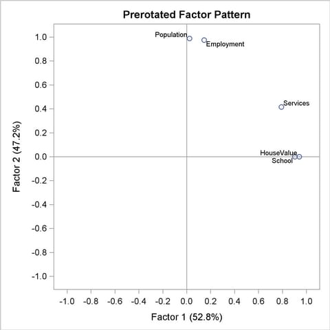
Output 33.2.6 and Output 33.2.7 display the results of the varimax rotation. This rotation puts one axis through the variables HouseValue and School but misses the Population and Employment variables slightly.
| Orthogonal Transformation Matrix | ||
|---|---|---|
| 1 | 2 | |
| 1 | 0.78895 | 0.61446 |
| 2 | -0.61446 | 0.78895 |
| Rotated Factor Pattern | ||
|---|---|---|
| Factor1 | Factor2 | |
| HouseValue | 0.94072 | -0.00004 |
| School | 0.90419 | 0.00055 |
| Services | 0.79085 | 0.41509 |
| Population | 0.02255 | 0.98874 |
| Employment | 0.14625 | 0.97499 |
| Final Communality Estimates: Total = 4.450370 | ||||
|---|---|---|---|---|
| Population | School | Employment | Services | HouseValue |
| 0.97811334 | 0.81756387 | 0.97199928 | 0.79774304 | 0.88494998 |
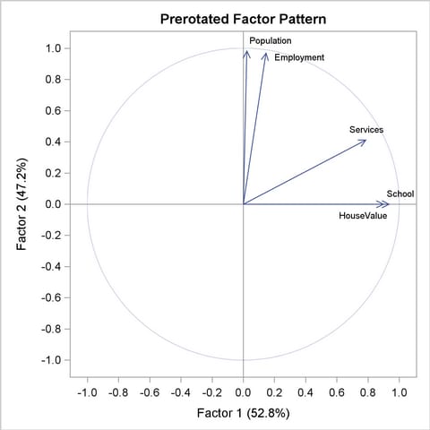
An alternative to the scatter plot of factor loadings as shown in Output 33.2.7 is the so-called vector plot of loadings. The vector plot is requested with the suboption VECTOR in the PLOTS= option. For example:
plots=preloadings(vector)
This will generate the vector plot of loadings as shown in Output 33.2.8.
The results of oblique promax rotation are shown in Output 33.2.9 and Output 33.2.10. The corresponding plot of factor loadings is shown in Output 33.2.11.
| Target Matrix for Procrustean Transformation | ||
|---|---|---|
| Factor1 | Factor2 | |
| HouseValue | 1.00000 | -0.00000 |
| School | 1.00000 | 0.00000 |
| Services | 0.69421 | 0.10045 |
| Population | 0.00001 | 1.00000 |
| Employment | 0.00326 | 0.96793 |
| Rotated Factor Pattern (Standardized Regression Coefficients) | ||
|---|---|---|
| Factor1 | Factor2 | |
| HouseValue | 0.95558485 | -0.0979201 |
| School | 0.91842142 | -0.0935214 |
| Services | 0.76053238 | 0.33931804 |
| Population | -0.0790832 | 1.00192402 |
| Employment | 0.04799 | 0.97509085 |
| Reference Structure (Semipartial Correlations) | ||
|---|---|---|
| Factor1 | Factor2 | |
| HouseValue | 0.93591 | -0.09590 |
| School | 0.89951 | -0.09160 |
| Services | 0.74487 | 0.33233 |
| Population | -0.07745 | 0.98129 |
| Employment | 0.04700 | 0.95501 |
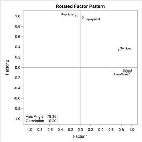
As shown in Output 33.2.11, the promax solution places an axis through the variables Population and Employment but misses the HouseValue and School variables. Since an independent-cluster solution would be possible if it were not for the variable Services, a Harris-Kaiser rotation weighted by the Cureton-Mulaik technique could be used. Rather than reanalyze the entire problem with the Harris-Kaiser rotation, you can simply use the preceding results stored in the OUTSTAT= data set.
First, the OUTSTAT= data set is printed using this code:
   title3 'Factor Output Data Set';
   proc print data=fact_all;
   run;
The output data set is displayed in Output 33.2.12.
| Five Socioeconomic Variables |
| See Page 14 of Harman: Modern Factor Analysis, 3rd Ed |
| Factor Output Data Set |
| Obs | _TYPE_ | _NAME_ | Population | School | Employment | Services | HouseValue |
|---|---|---|---|---|---|---|---|
| 1 | MEAN | 6241.67 | 11.4417 | 2333.33 | 120.833 | 17000.00 | |
| 2 | STD | 3439.99 | 1.7865 | 1241.21 | 114.928 | 6367.53 | |
| 3 | N | 12.00 | 12.0000 | 12.00 | 12.000 | 12.00 | |
| 4 | CORR | Population | 1.00 | 0.0098 | 0.97 | 0.439 | 0.02 |
| 5 | CORR | School | 0.01 | 1.0000 | 0.15 | 0.691 | 0.86 |
| 6 | CORR | Employment | 0.97 | 0.1543 | 1.00 | 0.515 | 0.12 |
| 7 | CORR | Services | 0.44 | 0.6914 | 0.51 | 1.000 | 0.78 |
| 8 | CORR | HouseValue | 0.02 | 0.8631 | 0.12 | 0.778 | 1.00 |
| 9 | COMMUNAL | 0.98 | 0.8176 | 0.97 | 0.798 | 0.88 | |
| 10 | PRIORS | 0.97 | 0.8223 | 0.97 | 0.786 | 0.85 | |
| 11 | EIGENVAL | 2.73 | 1.7161 | 0.04 | -0.025 | -0.07 | |
| 12 | UNROTATE | Factor1 | 0.63 | 0.7137 | 0.71 | 0.879 | 0.74 |
| 13 | UNROTATE | Factor2 | 0.77 | -0.5552 | 0.68 | -0.158 | -0.58 |
| 14 | RESIDUAL | Population | 0.02 | -0.0112 | 0.01 | 0.011 | 0.00 |
| 15 | RESIDUAL | School | -0.01 | 0.1824 | 0.02 | -0.024 | 0.01 |
| 16 | RESIDUAL | Employment | 0.01 | 0.0215 | 0.03 | -0.006 | -0.02 |
| 17 | RESIDUAL | Services | 0.01 | -0.0239 | -0.01 | 0.202 | 0.03 |
| 18 | RESIDUAL | HouseValue | 0.00 | 0.0125 | -0.02 | 0.034 | 0.12 |
| 19 | PRETRANS | Factor1 | 0.79 | -0.6145 | . | . | . |
| 20 | PRETRANS | Factor2 | 0.61 | 0.7889 | . | . | . |
| 21 | PREROTAT | Factor1 | 0.02 | 0.9042 | 0.15 | 0.791 | 0.94 |
| 22 | PREROTAT | Factor2 | 0.99 | 0.0006 | 0.97 | 0.415 | -0.00 |
| 23 | TRANSFOR | Factor1 | 0.74 | -0.7055 | . | . | . |
| 24 | TRANSFOR | Factor2 | 0.54 | 0.8653 | . | . | . |
| 25 | FCORR | Factor1 | 1.00 | 0.2019 | . | . | . |
| 26 | FCORR | Factor2 | 0.20 | 1.0000 | . | . | . |
| 27 | PATTERN | Factor1 | -0.08 | 0.9184 | 0.05 | 0.761 | 0.96 |
| 28 | PATTERN | Factor2 | 1.00 | -0.0935 | 0.98 | 0.339 | -0.10 |
| 29 | RCORR | Factor1 | 1.00 | -0.2019 | . | . | . |
| 30 | RCORR | Factor2 | -0.20 | 1.0000 | . | . | . |
| 31 | REFERENC | Factor1 | -0.08 | 0.8995 | 0.05 | 0.745 | 0.94 |
| 32 | REFERENC | Factor2 | 0.98 | -0.0916 | 0.96 | 0.332 | -0.10 |
| 33 | STRUCTUR | Factor1 | 0.12 | 0.8995 | 0.24 | 0.829 | 0.94 |
| 34 | STRUCTUR | Factor2 | 0.99 | 0.0919 | 0.98 | 0.493 | 0.09 |
This output data set can be used for Harris-Kaiser rotation by deleting observations with _TYPE_=’PATTERN’ and _TYPE_=’FCORR’, which are for the promax-rotated factors, and changing _TYPE_=’UNROTATE’ to _TYPE_=’PATTERN’. In this way, the initial orthogonal factor pattern matrix is saved in the observations with _TYPE_=’PATTERN’. The following factor analysis will then read in the factor pattern in the fact2 data set as an initial factor solution, which will then be rotated by the Harris-Kaiser rotation with Cureton-Mulaik weights.
The following statements produce Output 33.2.13:
   data fact2(type=factor);
      set fact_all;
      if _TYPE_ in('PATTERN' 'FCORR') then delete;
      if _TYPE_='UNROTATE' then _TYPE_='PATTERN';
   ods graphics on;

   title3 'Harris-Kaiser Rotation with Cureton-Mulaik Weights';
   proc factor rotate=hk norm=weight reorder
        plots=loadings;
   run;

   ods graphics off;
The results of the Harris-Kaiser rotation are displayed in Output 33.2.13.
| Variable Weights for Rotation | ||||
|---|---|---|---|---|
| Population | School | Employment | Services | HouseValue |
| 0.95982747 | 0.93945424 | 0.99746396 | 0.12194766 | 0.94007263 |
| Rotated Factor Pattern (Standardized Regression Coefficients) | ||
|---|---|---|
| Factor1 | Factor2 | |
| HouseValue | 0.94048 | 0.00279 |
| School | 0.90391 | 0.00327 |
| Services | 0.75459 | 0.41892 |
| Population | -0.06335 | 0.99227 |
| Employment | 0.06152 | 0.97885 |
| Reference Structure (Semipartial Correlations) | ||
|---|---|---|
| Factor1 | Factor2 | |
| HouseValue | 0.93719 | 0.00278 |
| School | 0.90075 | 0.00326 |
| Services | 0.75195 | 0.41745 |
| Population | -0.06312 | 0.98880 |
| Employment | 0.06130 | 0.97543 |
| Factor Structure (Correlations) | ||
|---|---|---|
| Factor1 | Factor2 | |
| HouseValue | 0.94071 | 0.08139 |
| School | 0.90419 | 0.07882 |
| Services | 0.78960 | 0.48198 |
| Population | 0.01958 | 0.98698 |
| Employment | 0.14332 | 0.98399 |
| Final Communality Estimates: Total = 4.450370 | ||||
|---|---|---|---|---|
| Population | School | Employment | Services | HouseValue |
| 0.97811334 | 0.81756387 | 0.97199928 | 0.79774304 | 0.88494998 |
A plot of the rotated loadings is shown in Output 33.2.14.
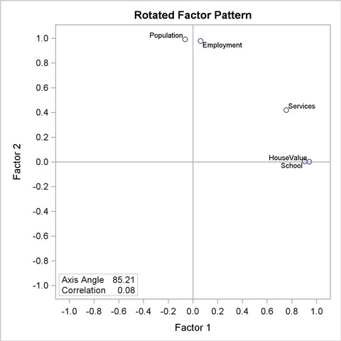
In the results of the Harris-Kaiser rotation, the variable Services receives a small weight, and the axes are placed as desired.
Copyright © 2009 by SAS Institute Inc., Cary, NC, USA. All rights reserved.