Project Description

The description is used to identify this particular project in the Open and Delete windows. Type a description for your project in the Project: text box.

For this example, change the description to Experimental blood pressure drug with two groups, as shown in Figure 68.35.

Solve For

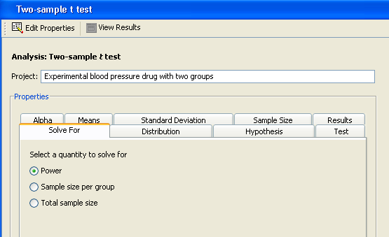
For the two-sample t test analysis, you can choose to solve for power, sample size per group, or total sample size. Specify the desired quantity type on the Solve For tab.

Click the Solve For tab and select the Power option as shown in Figure 68.35. For information about solving for sample size, see the section Solving for Sample Size.

Distribution

Click the Distribution tab to select a distribution option that specifies the underlying distribution for the test statistic, as shown in Figure 68.36.

Figure 68.36 Distribution Tab

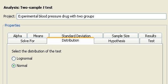
For this example, you are interested in means rather than mean ratios, so select the Normal option.

Hypothesis

Click the Hypothesis tab to select the type of test; see Figure 68.37.

Figure 68.37 Hypothesis Tab

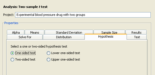
You can choose either a one- or two-sided test. If you do not know the direction of the effect (that is, whether it is positive or negative), the two-sided test is appropriate. If you know the effect’s direction, the one-sided test is appropriate. For the one-sided test, the alternative hypothesis is assumed to be in the same direction as the effect. If you specify a one-sided test and the effect is in the unexpected direction, the results of the analysis are invalid.

The One-sided test option assumes that you know the correct direction of the test. Select the Lower one-sided test and Upper one-sided test options to explicitly indicate the direction of the one-sided test.

Because you are interested only in whether the experimental drug lowers blood pressure, select the One-sided test option on the Hypothesis tab.

Test

Click the Test tab to select either the pooled t test or the Satterthwaite t test.

Figure 68.38 Test Tab

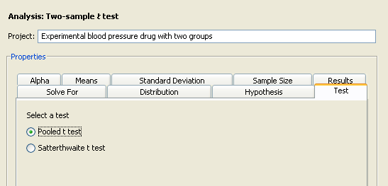
With the independent variances that the example uses, select Pooled t test option. The Satterthwaite t test is used with unequal variances; it is available only with the normal distribution.

Alpha

Click the Alpha tab to specify one or more significance levels, as shown in Figure 68.39.

Figure 68.39 Alpha Tab

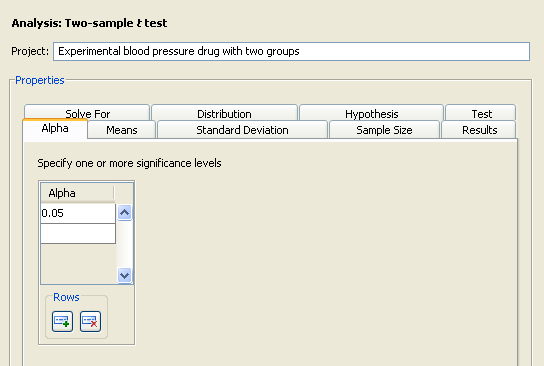
Alpha is the significance level (that is, the probability of falsely rejecting the null hypothesis). If you frequently use the same values for alpha, set them as defaults in the Preferences window. See the section Setting Preferences for more information about setting preferences.

Type the desired significance level of 0.05 in the first cell of the Alpha table (if it is not already the default value).

Means

Click the Means tab to select one of four possible ways to enter the means and the null mean difference, as shown in Figure 68.40.

Figure 68.40 Means Tab

Select one of the following forms from the Select A Form list. The four available forms are:

Difference between means

Enter the difference between the group means. The null mean difference is assumed to be 0.

Group means

Enter the means for each group. The null mean difference is assumed to be 0. The difference is formed by subtracting the mean for group 1 from the mean for group 2.

Difference between means, Null difference

Enter the difference between the group means and a null mean difference.

Group means, Null difference

Enter the means for each group and a null mean difference. The difference is formed by subtracting the mean for group 1 from the mean for group 2.

For this analysis, you can enter the means for the two groups either individually or as a difference. If your null mean difference is not zero, enter that value in the Null Mean table. (The Null Mean table is displayed only for the Group means, Null Difference and Difference between means, Null difference forms.)

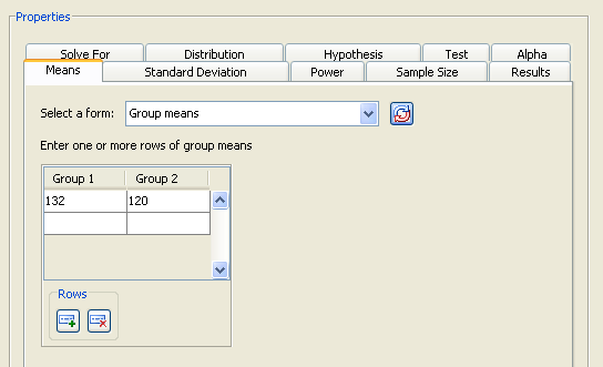
For this example, a null mean difference of 0 is reasonable, so select the Group means form from the list, as shown in Figure 68.40. Enter the control mean of 132 in the first row of the first column and the experimental mean of 120 in the first row of the second column.

Standard Deviation

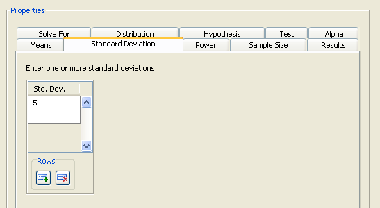
Click the Standard Deviation tab to enter the standard deviation for the two groups. It is assumed to be equal for both groups.

For the example, enter a single value of 15, as shown in Figure 68.41.

Figure 68.41 Standard Deviation Tab

Sample Size

Click the Sample Size tab to select one of three possible ways to enter the sample sizes, as shown in Figure 68.40.

Select one of the following forms from the Select A Form list:

Sample size per group

Enter the sample size for one of the two groups. The group sizes are assumed to be equal.

Group sample sizes

Enter the sample size for each of the two groups. The group sizes can be equal or unequal.

Total N, Group weights

Enter the total sample size for the two groups and the relative sample sizes for each group. For more information about using relative sample sizes, see the section Using Unequal Group Sizes.

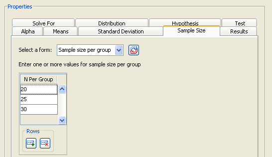
Examine the alternatives by clicking the Select a form down arrow. For this example, select the Sample size per group form. You want to examine a curve of powers in the power by sample size graph, so enter the values 20, 25, and 30 in the Sample Size table, as shown in Figure 68.42. If you need to add more rows to the table, add them by clicking the button beneath the table.

Figure 68.42 Sample Size Tab

Summary of Properties

Table 68.2 contains the values of the input parameters for the example.

Results

Click the Results tab to request desired results. Summary table and power by sample size graph options are available.

For the example, select the Create summary table and Create power by sample size graph check boxes.

Click Calculate to perform the analysis. If there are no errors in the input values, the View Results page appears. If there are errors in the input parameter values, you are prompted to correct them.

Summary Table

Click the Summary Table tab to view a table that includes the values of the input parameters and the computed quantity (in this example, power). See Figure 68.43.

Figure 68.43 Results Page with Summary Table

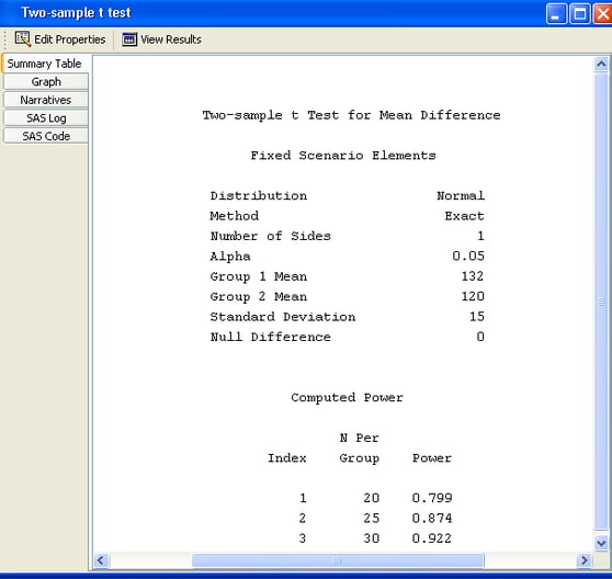
The table consists of two subtables: the Fixed Scenario Elements table that contains the input parameters that have only one value for the analysis, and the Computed Power table that contains the input parameters that have more than one value for the analysis and the corresponding power. Only the N per group parameter appears in the Computed Power table; all of the other input parameters have a single value. The computed power for a sample size per group of 25 is 0.874. Thus, you have a probability of 0.87 that the study will find the expected result if the assumptions and conjectured values are correct.

Power by Sample Size Graph

Click the Graph tab to view a power by sample size graph that displays power on the vertical axis and sample size per group on the horizontal axis. See Figure 68.44.

Figure 68.44 Power by Sample Size Graph

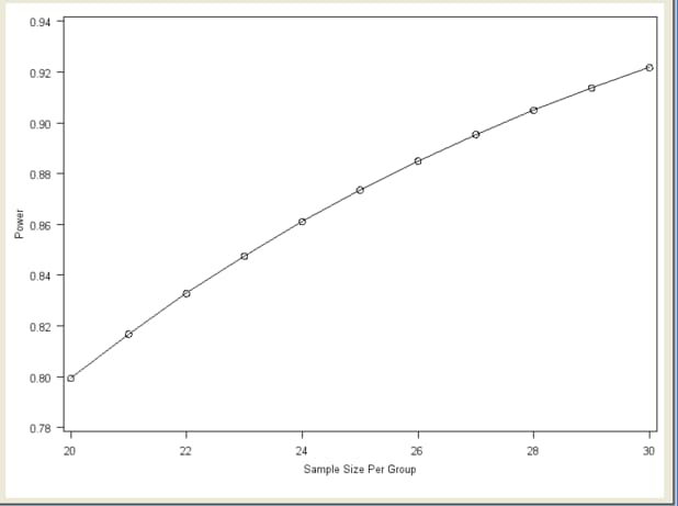
The range of values for the horizontal axis is 20 to 30, which were the smallest and largest values, respectively, that you entered on the Sample Size tab. You can customize the graph by specifying the values for the sample size axis (see the section Customizing Graphs).

Narratives

Click the Narratives tab to create and display a sentence- or paragraph-length text summary of the input parameter values and the computed quantity for combinations of the input parameter values; see Figure 68.45.

Figure 68.45 Narrative Selector and Display

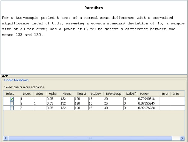
To create a narrative, selected the desired scenario (row) in the narrative selector table at the bottom of the Narratives tab.

In this example, select the narrative for the sample size per group of 20, which yields a power of 0.799. The following text summary is displayed:

For a two-sample pooled t test of a normal mean difference with a one-sided significance level of 0.05, assuming a common standard deviation of 15, a sample size of 20 per group has a power of 0.799 to detect a difference between the means 132 and 120.

To create other narratives, select the desired rows in the narrative selector table. If you also select the second row for the sample size of 25, another text summary is displayed below the first one:

For a two-sample pooled t test of a normal mean difference with a one-sided significance level of 0.05, assuming a common standard deviation of 15, a sample size of 20 per group has a power of 0.799 to detect a difference between the means 132 and 120. For a two-sample pooled t test of a normal mean difference with a one-sided significance level of 0.05, assuming a common standard deviation of 15, a sample size of 25 per group has a power of 0.874 to detect a difference between the means 132 and 120.

To change some values of the analysis and rerun it, select the Edit Properties page, change the desired properties, and click the Calculate button again.