The HPFMM Procedure

Suppose that you observe realizations of a random variable Y, the distribution of which depends on an unobservable random variable S that has a discrete distribution. S can occupy one of k states, the number of which might be unknown but is at least known to be finite. Since S is not observable, it is frequently referred to as a latent variable.
Let ![]() denote the probability that S takes on state j. Conditional on
denote the probability that S takes on state j. Conditional on ![]() , the distribution of the response Y is assumed to be
, the distribution of the response Y is assumed to be ![]() . In other words, each distinct state j of the random variable S leads to a particular distributional form
. In other words, each distinct state j of the random variable S leads to a particular distributional form ![]() and set of parameters
and set of parameters ![]() for Y.
for Y.
Let ![]() denote the collection of
denote the collection of ![]() and
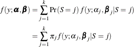
and ![]() parameters across all j = 1 to k. The marginal distribution of Y is obtained by summing the joint distribution of Y and S over the states in the support of S:
parameters across all j = 1 to k. The marginal distribution of Y is obtained by summing the joint distribution of Y and S over the states in the support of S:
This is a mixture of distributions, and the ![]() are called the mixture (or prior) probabilities. Because the number of states k of the latent variable S is finite, the entire model is termed a finite mixture (of distributions) model.
are called the mixture (or prior) probabilities. Because the number of states k of the latent variable S is finite, the entire model is termed a finite mixture (of distributions) model.
The finite mixture model can be expressed in a more general form by representing ![]() and
and ![]() in terms of regressor variables and parameters with optional additional scale parameters for
in terms of regressor variables and parameters with optional additional scale parameters for ![]() . The section Notation for the Finite Mixture Model develops this in detail.
. The section Notation for the Finite Mixture Model develops this in detail.