Data Input, Collection, and Analysis
Each block that collects data provides an output port (labeled OutData or OutCollected for the Number Holder block) that other blocks can use to access its data model object. The plot blocks (Histogram and Scatterplot, for example) are the usual recipients of these data; these blocks can provide real-time data analysis while the simulation is running. Typically, however, you also want to use SAS or JMP software to analyze the data that you have saved to data sets during a simulation run. The following sections provide an overview of output analysis options that are available within Simulation Studio, including the process for computing statistics for time-dependent and time-independent data, analysis techniques for terminating and steady-state simulations, and the use of the SAS block for data analysis and report generation.
Data that are collected during a simulation run can be used to estimate the parameters (such as the mean and variance) of the underlying population from which the data are sampled. For example, consider the population of waiting times for a particular queue. The waiting time data that are collected during a simulation run represent a sample from the population that consists of all possible waiting times. When you estimate population parameters from sample data, you need to consider two classifications of statistics:
-
For observation-based statistics, the data collected and used to estimate parameters are time-independent so that there is interest only in the observed value and not in when it was collected. Waiting-time data are an example of a time-independent sample, and the average waiting time is an example of an observation-based statistic. The following formula can be used to compute the average waiting time:
 , where
  are the set of n observed waiting times.
-
For time-persistent statistics, the data collected are time-dependent and it is necessary to record both the values and the time periods for which each value persisted. Queue length data are an example of a time-dependent sample, and the average queue length is an example of a time-persistent statistic. To compute the average queue length
 , the following formula is used:
  , where T is the total time period observed and
  is the number in the queue at time t. The average queue length is a weighted average of the possible queue lengths, where the weights are the amount of time that
a particular queue length value is observed. Another example of a time-dependent sample is the number of busy cashiers in
a store, and the average utilization of the cashiers is an example of a time-persistent statistic.
is the number in the queue at time t. The average queue length is a weighted average of the possible queue lengths, where the weights are the amount of time that
a particular queue length value is observed. Another example of a time-dependent sample is the number of busy cashiers in
a store, and the average utilization of the cashiers is an example of a time-persistent statistic.
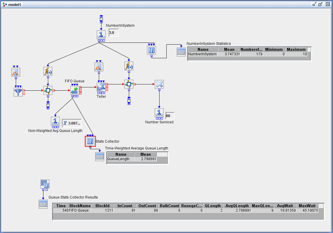
You can use the data collection blocks described in the section Block Data Storage to collect both time-dependent and time-independent data and, in some cases, to compute statistics. The Bucket block collects data—namely, the specified attributes of all entities that pass through the block along with the time that the attributes were recorded. However, the Bucket block does not compute statistics for those data. The Queue Stats and Server Stats Collector blocks collect data that are related to specific Queue or Server blocks in the model and automatically compute summary statistics such as average queue length, average waiting time, and average utilization. The Resource Stats Collector block can compute user-defined, time-persistent statistics for specific groups of resource entities. The Stats Collector block can compute statistics for any time-dependent or time-independent data that are generated by a model. For example, as shown in the simple bank system example in Figure 12.5, you can use a Number Holder block (labeled NumberInSystem) connected to a Stats Collector block to record data about the total number of customers in a bank. Each time the value in the Number Holder block is updated, that value and the current time are stored by the Stats Collector block. At the end of the run, the Stats Collector block computes the user-defined time-average number in the system, as displayed in the table labeled NumberInSystem Statistics.
Although you can use the Number Holder block to collect time-independent data and compute observation-based statistics (such
as mean, minimum, and maximum), you should not use the Number Holder block to compute statistics for time-dependent data.
In Figure 12.5, a Number Holder block labeled Non-WeightedAvgQueueLength is connected to the OutLength port of the FIFO Queue block and
the Display option in the Number Holder block is set to Mean. The average queue length computed by the Number Holder block is not time-weighted. The correct time-weighted average queue
length is computed by connecting a Stats Collector block to the OutLength port of the FIFO Queue block. This mean value, in
the table labeled Time-Weighted Average Queue Length in Figure 12.5, matches the value AvgQLength that is computed by the Queue Stats Collector block, as displayed in the table labeled Queue
Stats Collector Results.
For some systems, a clear and logical time determines the duration of the simulation run. For example, a doctor’s office might
be open from 8:00 a.m. until 5:00 p.m. Monday through Friday. If you are interested in estimating the average time that a
patient waits to see a doctor, then you can run the simulation for nine hours, which corresponds to the length of one day.
This type of simulation is called a terminating simulation. On the other hand, some systems have no clear end time. For example, you might be interested in estimating the
long-run average throughput for a manufacturing facility that operates 12 hours a day, with the work in process carried over
to the next day. This type of simulation is called a nonterminating (steady-state) simulation. In general, you are interested in the long-run behavior of the system while it is operating normally. Let ![]() denote a stochastic process that represents the sequence of outputs that are generated by a single run of a steady-state
simulation. For example, the random variable
denote a stochastic process that represents the sequence of outputs that are generated by a single run of a steady-state
simulation. For example, the random variable ![]() might represent the time in the system (cycle time) for the ith piece of work to complete all its processing in a simulation of a production facility. If the simulation is in steady-state
operation, then the random variables
might represent the time in the system (cycle time) for the ith piece of work to complete all its processing in a simulation of a production facility. If the simulation is in steady-state
operation, then the random variables ![]() have the same steady-state cumulative distribution function
have the same steady-state cumulative distribution function ![]() for all real x and for
for all real x and for ![]() .
.
Typically the data for a particular output process that are collected during a single terminating or steady-state simulation
run are neither independent nor identically distributed (iid); therefore, classic statistical methods (such as those for computing
point and confidence interval estimators) are not applicable. For example, in the bank system model in Figure 12.5, the individual observed waiting times for customers ![]() that are collected during a single simulation run are nonstationary and autocorrelated. Since the requirement of iid observations
is violated, you should not use the data
that are collected during a single simulation run are nonstationary and autocorrelated. Since the requirement of iid observations
is violated, you should not use the data ![]() from a single simulation run to compute, for example, a confidence interval for the average waiting time at the bank.
from a single simulation run to compute, for example, a confidence interval for the average waiting time at the bank.
For a terminating simulation, suppose that you run k independent replications of the same simulation model so that each replication uses the same initial conditions and a different
set of random numbers. Furthermore, you define a response or performance measure, such as the average waiting time, so that
for each replication a single value is collected. Then the observed k responses are iid and classic statistical methods can be applied to analyze the data. For example, suppose k replications of the bank system model are run and the average customer waiting time ![]() is computed for each replication j. A statistically valid point estimate of the mean waiting time in the bank system can then be computed as
is computed for each replication j. A statistically valid point estimate of the mean waiting time in the bank system can then be computed as ![]() .
.
For terminating simulations, the Experiment window provides the most straightforward method for collecting data and computing basic statistics for defined responses. By default, the Experiment window reports the average response over all replications for each design point. But you can also display the standard deviation, minimum value, or maximum value by right-clicking the column heading for a particular response and selecting the Summary menu item. Furthermore, by default each random stream in the model advances to its next substream at the start of a new replication. This guarantees that different random numbers are used for each replication. Alternatively, you can run multiple replications of a model, use the various data collection blocks to collect data for each replication, and then use SAS or JMP to analyze the data.
As in the case of a terminating simulation, the observations ![]() from a single long run of a nonterminating simulation are usually correlated. Furthermore, it is usually impossible to start
a simulation in steady-state operation. Thus, it is necessary to decide how long the warm-up period should be so that for
each simulation output that is generated after the end of the warm-up period, the corresponding expected value is sufficiently
close to the steady-state mean. If observations that are generated before the end of the warm-up period are included in the
analysis, then any computed point estimator (such as for the steady-state mean) might be biased. You could use a replication/deletion
approach to analyze data from a steady-state simulation, similar to the replication method used in the terminating simulation
case. You would first make k replications of the simulation, each of length n, and delete the first l observations from each replication. You would then compute the truncated sample mean for each replication as
from a single long run of a nonterminating simulation are usually correlated. Furthermore, it is usually impossible to start
a simulation in steady-state operation. Thus, it is necessary to decide how long the warm-up period should be so that for
each simulation output that is generated after the end of the warm-up period, the corresponding expected value is sufficiently
close to the steady-state mean. If observations that are generated before the end of the warm-up period are included in the
analysis, then any computed point estimator (such as for the steady-state mean) might be biased. You could use a replication/deletion
approach to analyze data from a steady-state simulation, similar to the replication method used in the terminating simulation
case. You would first make k replications of the simulation, each of length n, and delete the first l observations from each replication. You would then compute the truncated sample mean for each replication as ![]() for
for ![]() . By deleting those observations at the beginning of the simulation runs, you eliminate the initial bias due to the model’s
initial conditions. The replication/deletion method is simple to understand and implement. However, it is computationally
inefficient because it requires the deletion of a total of
. By deleting those observations at the beginning of the simulation runs, you eliminate the initial bias due to the model’s
initial conditions. The replication/deletion method is simple to understand and implement. However, it is computationally
inefficient because it requires the deletion of a total of ![]() observations. In addition, it can be difficult to determine how large the warm-up period l should be.
observations. In addition, it can be difficult to determine how large the warm-up period l should be.
An alternate method to replication/deletion for analyzing data from a steady-state simulation is to make one long simulation run of length n and apply a batch means approach. The Steady State block in Simulation Studio provides an automated batch means method for producing a statistically valid confidence interval estimator for a steady-state mean response in a nonterminating simulation model where the delivered confidence interval satisfies a user-specified precision requirement. The procedure is based on the method of spaced batch means and has an algorithm built in to automatically detect the end of the warm-up period and to address the correlation that exists between observations. For more information about the specific batch means method used by the Steady State block, see Lada, Steiger, and Wilson (2008). For more information about using the Steady State block specifically, see Appendix A: Templates.
The SAS Program block enables you to execute a SAS program or JMP script at any point during a simulation run. This enables you to analyze simulation-generated data automatically either at the end of a run (see the example Using the SAS Program Block to Analyze Simulation Results) or during a run by sending a signal to the InSubmitCode port of the SAS Program block. For example, in a simulation model of an inventory system it might be necessary, based on the current state of the system, to update a production plan data set. If the number of backlogged orders exceeds a certain level, a SAS Program block can be signaled to execute a program that generates a new production plan data set that is used to set production levels downstream in the model.