Multiple Regression

Creating the Analysis

The GPA data set contains data collected to determine which applicants at a large midwestern university were likely to succeed in its computer science program. The variable GPA is the measure of success of students in the computer science program, and it is the response variable. A response variable measures the outcome to be explained or predicted.

Several other variables are also included in the study as possible explanatory variables or predictors of GPA. An explanatory variable may explain variation in the response variable. Explanatory variables for this example include average high school grades in mathematics (HSM), English (HSE), and science (HSS) (Moore and McCabe 1989).

To begin the regression analysis, follow these steps.

Open the GPA data set.

Choose Analyze:Fit (Y X).

[menu]
Figure 14.2: Analyze Menu

The fit variables dialog appears, as shown in Figure 14.3. This dialog differs from all other variables dialogs because it can remain visible even after you create the fit window. This makes it convenient to add and remove variables from the model. To make the variables dialog stay on the display, click on the Apply button when you are finished specifying the model. Each time you modify the model and use the Apply button, a new fit window appears so you can easily compare models. Clicking on OK also displays a new fit window but closes the dialog.

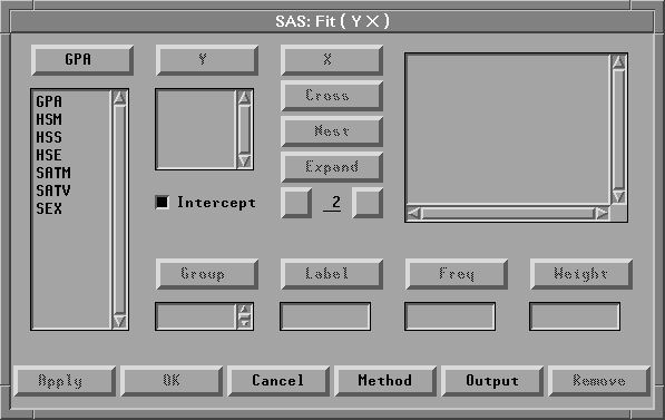
Figure 14.3: Fit Variables Dialog

Select the variable GPA in the list on the left, then click the Y button.

GPA appears in the Y variables list.

Select the variables HSM, HSS, and HSE, then click the X button.

HSM, HSS, and HSE appear in the X variables list.

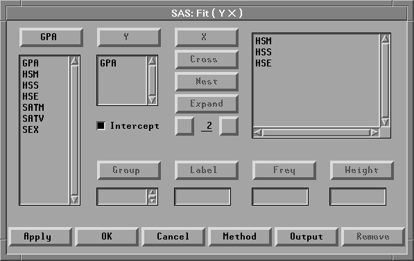
Figure 14.4: Variable Roles Assigned

Click the Apply button.

A fit window appears, as shown in Figure 14.5.

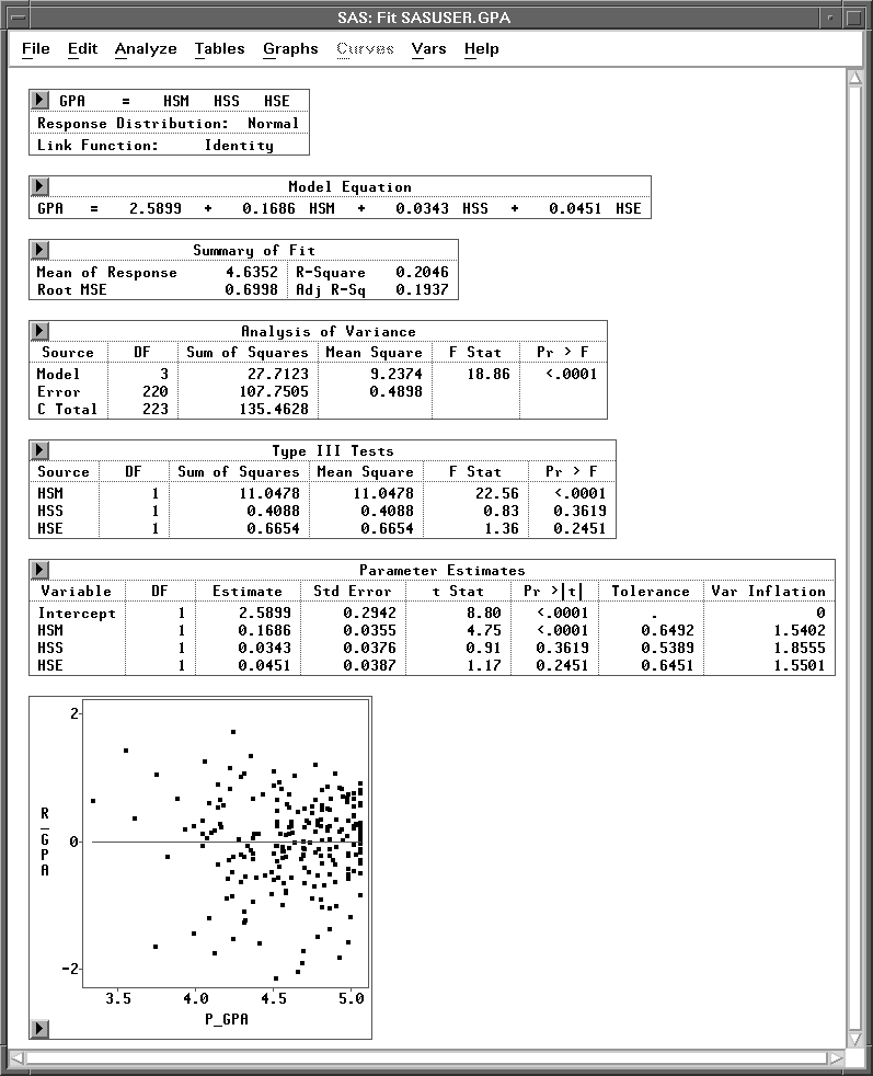
Figure 14.5: Fit Window

This window shows the results of a regression analysis of GPA on HSM, HSS, and HSE. The regression model for the ith observation can be written as

${GPA}_{i} = {\beta}_{0} + {\beta}_{1} {HSM}_{i} + {\beta}_{2} {HSS}_{i} + {\beta}_{3} {HSE}_{i} + {\epsilon}_{i}$

where GPA_i is the value of GPA; ${ {\beta}_{0}}$ to ${ {\beta}_{3}}$ are the regression coefficients (parameters); HSM_i, HSS_i, and HSE_i are the values of the explanatory variables; and ${ {\epsilon}_{i}}$ is the random error term. The ${ {\epsilon}_{i}}$ 's are assumed to be uncorrelated, with mean 0 and variance ${ {\sigma}^2}$ .

By default, the fit window displays tables for model information, Model Equation, Summary of Fit, Analysis of Variance, Type III Tests, and Parameter Estimates, and a residual-by-predicted plot, as illustrated in Figure 14.5. You can display other tables and graphs by clicking on the Output button on the fit variables dialog or by choosing menus as described in the section "Adding Tables and Graphs" later in this chapter.

Creating the Analysis

Model Information

Summary of Fit

Analysis of Variance

Type III Tests

Parameter Estimates

Residuals-by-Predicted Plot