| Fit Analyses |
Output
To view or change the options associated with your fit analysis, click the Output button in the variables dialog. This displays the output options dialog shown in Figure 39.4.
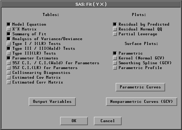
Figure 39.4: Fit Output Options Dialog
The options you set in this dialog determine the tables and graphs that appear in the fit window. Provided by default are tables of the model equation, summary of fit, analysis of variance or deviance, type III or type III (Wald) tests, and parameter estimates and a plot of residuals by predicted values.
When there are two explanatory variables in the model, a parametric response surface plot is created by default. You can also generate a nonparametric kernel or a thin-plate smoothing spline response surface plot. With more than two explanatory variables in the model, a parametric profile response surface plot with the first two explanatory variables can be created. The values of the remaining explanatory variables are set to their corresponding means in the plot. You can use the sliders to change these values of the remaining explanatory variables.
Click on the Output Variables button in the fit dialog to display the Output Variables dialog shown in Figure 39.5. The Output Variables dialog enables you to specify variables that can be saved in the data window. Output variables include predicted values and several influence diagnostic variables based on the model you fit.
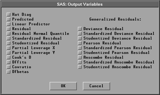
Figure 39.5: Output Variables Dialog
When there is only one explanatory variable in the model, a Y-by-X scatter plot is generated. The Parametric Curves and Nonparametric Curves (GCV) buttons display dialogs that enable you to fit parametric and nonparametric curves to this scatter plot.
Click on Parametric Curves to display the Parametric Curves dialog.
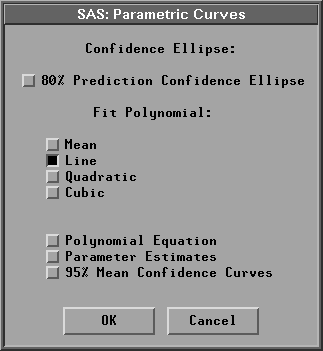
Figure 39.6: Parametric Curves Dialog
A regression line fit is provided by default. You can request an 80% prediction ellipse and other polynomial fits in the dialog. You can also request polynomial equation tables, parameter estimates tables, and 95% mean confidence curves for fitted polynomials.
The Nonparametric Curves (GCV) dialog in Figure 39.7 includes a smoothing spline, a kernel smoother, and a local polynomial smoother. You must specify the method, regression type, and weight function for a local polynomial fit.
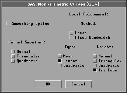
Figure 39.7: Nonparametric Curves Dialog
Copyright © 2007 by SAS Institute Inc., Cary, NC, USA. All rights reserved.