QQPLOT Statement: CAPABILITY Procedure

Note: See Creating Lognormal Q-Q Plots in the SAS/QC Sample Library.

The following statements produce the normal Q-Q plot in Output 5.21.1:

data Measures;
   input Diameter @@;
   label Diameter='Diameter in mm';
   datalines;
5.501  5.251  5.404  5.366  5.445  5.576  5.607
5.200  5.977  5.177  5.332  5.399  5.661  5.512
5.252  5.404  5.739  5.525  5.160  5.410  5.823
5.376  5.202  5.470  5.410  5.394  5.146  5.244
5.309  5.480  5.388  5.399  5.360  5.368  5.394
5.248  5.409  5.304  6.239  5.781  5.247  5.907
5.208  5.143  5.304  5.603  5.164  5.209  5.475
5.223
 ;

title 'Normal Q-Q Plot for Diameters';
proc capability data=Measures noprint;
   qqplot Diameter / normal square odstitle=title;
run;

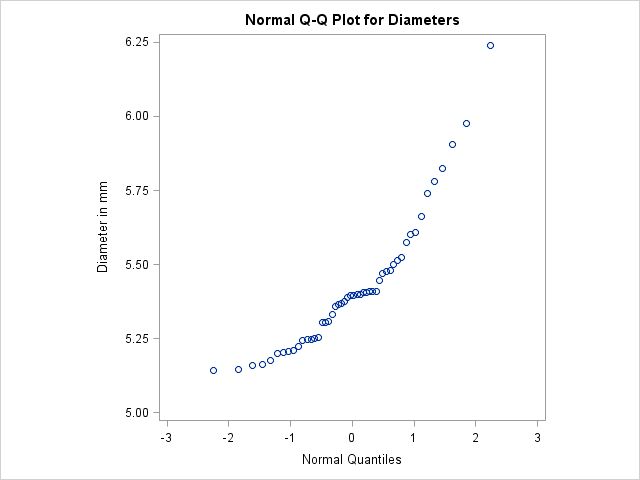
The nonlinearity of the points in Output 5.21.1 indicates a departure from normality. Because the point pattern is curved with slope increasing from left to right, a theoretical distribution that is skewed to the right, such as a lognormal distribution, should provide a better fit than the normal distribution. The mild curvature suggests that you should examine the data with a series of lognormal Q-Q plots for small values of the shape parameter, as illustrated in the next example.