HISTOGRAM Statement: CAPABILITY Procedure

Example 5.14 Annotating a Folded Normal Curve
Note: See Cpk for Folded Normal Distribution in the SAS/QC Sample Library.
This example shows how to display a fitted curve that is not supported by the HISTOGRAM statement.
The offset of an attachment point is measured (in mm) for a number of manufactured assemblies, and the measurements are saved
in a data set named Assembly.
data Assembly;
   label Offset = 'Offset (in mm)';
   input Offset @@;
   datalines;
11.11 13.07 11.42  3.92 11.08  5.40 11.22 14.69  6.27  9.76
 9.18  5.07  3.51 16.65 14.10  9.69 16.61  5.67  2.89  8.13
 9.97  3.28 13.03 13.78  3.13  9.53  4.58  7.94 13.51 11.43
11.98  3.90  7.67  4.32 12.69  6.17 11.48  2.82 20.42  1.01
 3.18  6.02  6.63  1.72  2.42 11.32 16.49  1.22  9.13  3.34
 1.29  1.70  0.65  2.62  2.04 11.08 18.85 11.94  8.34  2.07
 0.31  8.91 13.62 14.94  4.83 16.84  7.09  3.37  0.49 15.19
 5.16  4.14  1.92 12.70  1.97  2.10  9.38  3.18  4.18  7.22
15.84 10.85  2.35  1.93  9.19  1.39 11.40 12.20 16.07  9.23
 0.05  2.15  1.95  4.39  0.48 10.16  4.81  8.28  5.68 22.81
 0.23  0.38 12.71  0.06 10.11 18.38  5.53  9.36  9.32  3.63
12.93 10.39  2.05 15.49  8.12  9.52  7.77 10.70  6.37  1.91
 8.60 22.22  1.74  5.84 12.90 13.06  5.08  2.09  6.41  1.40
15.60  2.36  3.97  6.17  0.62  8.56  9.36 10.19  7.16  2.37
12.91  0.95  0.89  3.82  7.86  5.33 12.92  2.64  7.92 14.06
;
The assembly process is in statistical control, and it is decided to fit a folded normal distribution to the offset measurements. A variable X has a folded normal distribution if  , where Y is distributed as
  . The fitted density is
![\[ h(x) = \frac{1}{\sqrt {2\pi } \sigma } \left[ \exp \left( -\frac{(x-\mu )^2}{2\sigma ^2} \right) + \exp \left( -\frac{(x+\mu )^2}{2\sigma ^2} \right) \right] \; \; \; \; \; , \; x \geq 0 \]](images/qcug_capability0493.png)
You can use SAS/IML software to compute preliminary estimates of  and
and  based on a method of moments given by Elandt (1961). These estimates are computed by solving equation (19) of Elandt (1961), which is given by
![\[ f(\theta ) = \frac{\left( \frac{2}{\sqrt {2\pi }} e^{-\theta ^2/2 } - \theta \left[ 1-2\Phi (\theta ) \right] \right)^2}{1+\theta ^2} = A \]](images/qcug_capability0494.png)
where  is the standard normal distribution function, and
![\[ A = \frac{ \bar{x}^2 }{ \frac{1}{n} \sum _{i=1}^ n x_ i^2 } \]](images/qcug_capability0495.png)
Then the estimates of and are given by
![\[ \begin{array}{lll} \hat{\sigma }_0 & = \sqrt { \frac{ \frac{1}{n} \sum _{i=1}^ n x_ i^2}{1 + \hat{\theta }^2 } } \\[.1in] \hat{\mu }_0 & = \hat{\theta } \cdot \hat{\sigma }_0 \end{array} \]](images/qcug_capability0496.png)
Begin by using the MEANS procedure to compute the first and second moments and using the DATA step to compute the constant A.
proc means data = Assembly noprint;
   var Offset;
   output out=Stat mean=m1 var=var n=n min = min;
run;

* Compute constant A from equation (19) of Elandt (1961) ;
data Stat;
   keep m2 a min;
   set Stat;
   a  = (m1*m1);
   m2 = ((n-1)/n)*var + a;
   a  = a/m2;
run;
Next, use the SAS/IML subroutine NLPDD to solve equation (19) by minimizing  , and compute
  and
and  .
.
proc iml;
   use Stat;
   read all var {m2}  into m2;
   read all var {a}   into a;
   read all var {min} into min;

   * f(t) is the function in equation (19) of Elandt (1961) ;
   start f(t) global(a);
      y = .39894*exp(-0.5*t*t);
      y = (2*y-(t*(1-2*probnorm(t))))**2/(1+t*t);
      y = (y-a)**2;
      return(y);
   finish;

   * Minimize (f(t)-A)**2 and estimate mu and sigma ;
   if ( min < 0 ) then do;
      print "Warning: Observations are not all nonnegative.";
      print "     The folded normal is inappropriate.";
      stop;
   end;
   if ( a < 0.637 ) then do;
      print "Warning: the folded normal may be inappropriate";
   end;
   opt = { 0 0 };
   con = { 1e-6 };
   x0  = { 2.0 };
   tc  = { . . . . . 1e-12 . . . . . . .};
   call nlpdd(rc,etheta0,"f",x0,opt,con,tc);
   esig0 = sqrt(m2/(1+etheta0*etheta0));
   emu0  = etheta0*esig0;

   create Prelim var {emu0 esig0 etheta0};
   append;
   close Prelim;
      * Define the log likelihood of the folded normal ;
      start g(p) global(x);
         y = 0.0;
         do i = 1 to nrow(x);
            z = exp( (-0.5/p[2])*(x[i]-p[1])*(x[i]-p[1]) );
            z = z + exp( (-0.5/p[2])*(x[i]+p[1])*(x[i]+p[1]) );
            y = y + log(z);
         end;
         y = y - nrow(x)*log( sqrt( p[2] ) );
         return(y);
      finish;
      * Maximize the log likelihood with subroutine NLPDD ;
      use Assembly;
      read all var {Offset} into x;
      esig0sq = esig0*esig0;
      x0      = emu0||esig0sq;
      opt     = { 1 0 };
      con     = { . 0.0, .  .  };
      call nlpdd(rc,xr,"g",x0,opt,con);
      emu     = xr[1];
      esig    = sqrt(xr[2]);
      etheta  = emu/esig;
      create Parmest var{emu esig etheta};
      append;
      close Parmest;
   quit;
title 'The Data Set Prelim';
proc print data=Prelim noobs;
run;
The preliminary estimates are saved in the data set Prelim, as shown in Output 5.14.1.
Output 5.14.1: Preliminary Estimates of , , and 
Now, using and as initial estimates, call the NLPDD subroutine to maximize the log likelihood,  , of the folded normal distribution, where, up to a constant,
![\[ l(\mu ,\sigma ) = -n \log \sigma + \sum _{i=1}^ n \log \left[ \exp \left( -\frac{(x_ i-\mu )^2}{2\sigma ^2} \right) + \exp \left( -\frac{(x_ i+\mu )^2}{2\sigma ^2} \right) \right] \]](images/qcug_capability0501.png)
   * Define the log likelihood of the folded normal ;
   start g(p) global(x);
      y = 0.0;
      do i = 1 to nrow(x);
         z = exp( (-0.5/p[2])*(x[i]-p[1])*(x[i]-p[1]) );
         z = z + exp( (-0.5/p[2])*(x[i]+p[1])*(x[i]+p[1]) );
         y = y + log(z);
      end;
      y = y - nrow(x)*log( sqrt( p[2] ) );
      return(y);
   finish;

   * Maximize the log likelihood with subroutine NLPDD ;
   use assembly;
   read all var {offset} into x;
   esig0sq = esig0*esig0;
   x0      = emu0||esig0sq;
   opt     = { 1 0 };
   con     = { . 0.0, .  .  };
   call nlpdd(rc,xr,"g",x0,opt,con);
   emu     = xr[1];
   esig    = sqrt(xr[2]);
   etheta  = emu/esig;

   create parmest var{emu esig etheta};
   append;
   close parmest;
quit;
title 'The Data Set PARMEST';
proc print data=Parmest noobs;
   var emu esig etheta;
run;
The data set Parmest saves the maximum likelihood estimates  and
and  (as well as
  ), as shown in Output 5.14.2.
Output 5.14.2: Final Estimates of , , and
To annotate the curve on a histogram, begin by computing the width and endpoints of the histogram intervals. The following statements save these values in an OUTFIT= data set called OUT. Note that a plot is not produced at this point.
ods graphics off;
proc capability data = Assembly noprint;
   histogram Offset / outfit = Out normal(noprint) noplot;
run;
title 'OUTFIT= Data Set Out';
proc print data=Out noobs round;
   var _var_ _curve_ _locatn_ _scale_ _chisq_ _df_ _pchisq_
       _midpt1_ _width_ _midptn_ _expect_ _eststd_ _adasq_
       _adp_ _cvmwsq_ _cvmp_ _ksd_ _ksp_;
run;
Output 5.14.3 provides a partial listing of the data set Out. The width and endpoints of the histogram bars are saved as values of the variables _WIDTH_, _MIDPT1_, and _MIDPTN_. See Output Data Sets.
Output 5.14.3: The OUTFIT= Data Set Out
The following statements create an annotate data set named Anno, which contains the coordinates of the fitted curve:
data Anno;
   merge Parmest Out;
   length function color $ 8;

   function = 'point';
   color    = 'black';
   size     =  2;
   xsys     = '2';
   ysys     = '2';
   when     = 'a';
   constant = 39.894*_width_;;
   left     =  _midpt1_ - .5*_width_;
   right    =  _midptn_ + .5*_width_;
   inc      = (right-left)/100;
   do x = left to right by inc;
      z1 = (x-emu)/esig;
      z2 = (x+emu)/esig;
      y  = (constant/esig)*(exp(-0.5*z1*z1)+exp(-0.5*z2*z2));
      output;
      function = 'draw';
   end;
run;
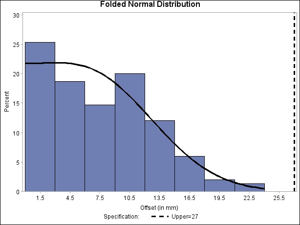
The following statements read the ANNOTATE= data set and display the histogram and fitted curve, as shown in Output 5.14.4:
ods graphics off;
title "Folded Normal Distribution";
proc capability data=Assembly noprint;
   spec usl=27 cusl=black lusl=2 wusl=2;
   histogram Offset / annotate = Anno;
run;
Output 5.14.4: Histogram with Annotated Folded Normal Curve