XCHART Statement: ANOM Procedure

Constructing ANOM Charts for Two-Way Layouts
This section provides the computational details for constructing an ANOM chart for the lth factor in an experiment involving two factors (l = 1 or 2). It is assumed that there is no interaction effect. See Example 4.5 for an illustration.
The following notation is used in this section:
|
|
kth response at the ith level of factor 1 and the jth level of factor 2, where |
|
|
Number of groups (levels) for the lth factor, |
|
|
Number of replicates in cell |
|
N |
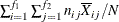
Total sample size |
|
|
Variance of a response |
|
|
Average response in cell |
|
|
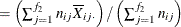
Average response for ith level of factor 1 |
|
|
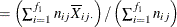
Average response for jth level of factor 2 |
|
|
|
|
|
Sample variance of the responses for the ith level of factor 1 and the jth level of factor 2 |
|
|
Mean square error (MSE) in the two-way analysis of variance |
|
|
Degrees of freedom associated with the mean square error in the two-way analysis of variance |
|
|
Significance level |
|
|
Critical value for analysis of means in a one-way layout for |


Plotted Points
The points on the ANOM chart for factor 1 represent  ,
,  and the points on the ANOM chart for factor 2 represent
  ,
,  .
.
Central Line
The central line on the ANOM chart for the lth factor is the overall weighted average  . Some authors use the notation
  for this average.
Decision Limits
It is assumed that
![\[ X_{ijk} = \mu + \alpha _{i} + \beta _{j} + \epsilon _{ijk} \]](images/qcug_anom0090.png)
where the quantities  are independent and at least approximately normally distributed with
![\[ \epsilon _{ijk} \sim N( 0, \sigma ^2 ) \; \; \; \; \; \]](images/qcug_anom0092.png)
The correct decision limits for a given factor in a two-way layout are not computed by default when the lth factor is specified as the group-variable in the XCHART statement, since the mean square error and degrees of freedom are not adjusted for the two-way structure of
the data. Consequently,  and
and  must be precomputed and provided to the ANOM procedure, as illustrated in Example 4.5.
In the case of a two-way layout with equal group sizes ( ), the appropriate decision limits are:
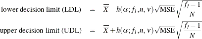
where the mean square error (MSE) is computed as in the ANOVA or GLM procedure:
![\[ \mbox{MSE} = \widehat{\sigma ^2} = \frac{1}{f_{1}f_{2}} \sum _{i=1}^{f_{1}} \sum _{j=1}^{f_{2}} s_{ij}^2 \]](images/qcug_anom0095.png)
and the degrees of freedom for error is  . For details concerning the function
  , see Nelson (1982a, 1993).
You can provide the appropriate values of MSE and by
-
specifying
with the MSE= option or with the variable _MSE_in a LIMITS= data set -
specifying
with the DFE= option or with the variable _DFE_in a LIMITS= data set
In addition you can:
-
Specify
 with the ALPHA= option or with the variable
 _ALPHA_in a LIMITS= data set. By default, .
.
-
Specify a constant nominal sample size
for the decision limits in the balanced case with the LIMITN= option or with the variable _LIMITN_in a LIMITS= data set. -
Specify
 with the LIMITK= option or with the variable
 _LIMITK_in a LIMITS= data set. -
Specify
with the MEAN= option or with the variable _MEAN_in a LIMITS= data set.