BOXCHART Statement: ANOM Procedure

Constructing ANOM Boxcharts

The following notation is used in this section:

$X_{ij}$	jth response in the ith group
k	Number of groups
$n_{i}$	Sample size of ith group
N	Total sample size $= n_1 + \cdots + n_ k$
$\mu _ i$	Expected value of a response in the ith group
$\sigma$	Standard deviation of response
$\bar{X}_{i}$	Average response in ith group
$\overline{\overline{X}}$	Weighted average of k group means
$s_{i}^{2}$	Sample variance of the responses in the ith group
$\widehat{\sigma ^2}$	Mean square error (MSE)
$\nu$	Degrees of freedom associated with the mean square error
$\alpha$	Significance level
$h(\alpha ; k, n, \nu )$	Critical value for analysis of means when the sample sizes $n_ i$ are equal $(n_ i \equiv n)$
$h(\alpha ; k, n_1,\ldots , n_ k, \nu )$	Critical value for analysis of means when the sample sizes $n_ i$ are not equal

Elements of Box-and-Whisker Plots

A box-and-whisker plot is displayed for the measurements in each group on the ANOM boxchart. Figure 4.9 illustrates the elements of each plot.

Figure 4.9: Box-and-Whisker Plot

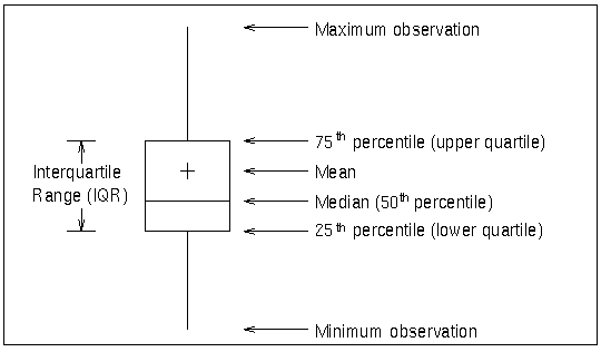
The skeletal style of the box-and-whisker plot shown in Figure 4.9 is the default. You can specify alternative styles with the BOXSTYLE= option; see the entry for the BOXSTYLE= option in Dictionary of Options: SHEWHART Procedure.

Central Line

By default, the central line on an ANOM chart for means represents the weighted average of the group means, which is computed as

$\overline{\overline{X}} = \frac{n_{1}\bar{X_{1}} + \cdots + n_{k}\bar{X_{k}}}{n_{1} + \cdots + n_{k}}$

You can specify a value for $\overline{\overline{X}}$ with the MEAN= option in the BOXCHART statement or with the variable _MEAN_ in a LIMITS= data set.

Decision Limits

In the analysis of means for continuous data, it is assumed that the responses in the ith group are at least approximately normally distributed with a constant variance:

$X_{ij} \sim N( \mu _{i}, \sigma ^2 ), \; \; \; \; \; j = 1, \ldots , n_ i$

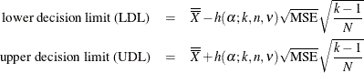
When the group sizes are constant 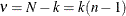( $n_ i \equiv n$ ), then $\nu = N-k=k(n-1)$ and the decision limits are computed as follows:

$\begin{eqnarray*} \mbox{lower decision limit (LDL)} & = & \overline{\overline{X}} - h(\alpha ; k, n, \nu ) \sqrt {\mbox{MSE}} \sqrt { \frac{k-1}{N}} \\ \mbox{upper decision limit (UDL)} & = & \overline{\overline{X}} + h(\alpha ; k, n, \nu ) \sqrt {\mbox{MSE}} \sqrt {\frac{k-1}{N}} \end{eqnarray*}$

Here the mean square error (MSE) is computed as follows:

$\mbox{MSE} = \widehat{\sigma ^2} = \frac{1}{k} \sum _{j=1}^{k} s_{j}^2$

For details concerning the function $h(\alpha ; k, n, \nu )$ , see Nelson (1981, 1982a, 1993).

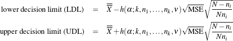
When the group sizes $n_ i$ are not constant (the unbalanced case), $\nu = N-k$ and the decision limits for the ith group are computed as follows:

$\begin{eqnarray*} \mbox{lower decision limit (LDL)} & = & \overline{\overline{X}} - h(\alpha ; k, n_1,\ldots ,n_ k, \nu ) \sqrt {\mbox{MSE}} \sqrt { \frac{N-n_ i}{Nn_ i}} \\ \mbox{upper decision limit (UDL)} & = & \overline{\overline{X}} + h(\alpha ; k, n_1,\ldots ,n_ k, \nu ) \sqrt {\mbox{MSE}} \sqrt {\frac{N - n_ i}{Nn_ i}} \end{eqnarray*}$

Here the mean square error (MSE) is computed as follows:

$\mbox{MSE} = \widehat{\sigma ^2} = \frac{(n_{1} - 1)s_1^{2} + \cdots + (n_{k} - 1)s_{k}^{2}}{n_{1} + \cdots + n_{k} - k}$

This requires that $\nu$ be positive. A chart is not produced if $\nu >0$ but MSE is equal to zero (unless you specify the ZEROSTD option). For details concerning the function $h(\alpha ; k, n_1,\ldots ,n_ k, \nu )$ , see Fritzsch and Hsu (1997), Nelson (1982b, 1991), and Soong and Hsu (1997).

You can specify parameters for the limits as follows:

Specify $\alpha$ with the ALPHA= option or with the variable _ALPHA_ in a LIMITS= data set. By default, $\alpha$ = 0.05.
Specify a constant nominal sample size $n_{i} \equiv n$ for the decision limits in the balanced case with the LIMITN= option or with the variable _LIMITN_ in a LIMITS= data set. By default, n is the observed sample size in the balanced case.
Specify k with the LIMITK= option or with the variable _LIMITK_ in a LIMITS= data set. By default, k is the number of groups.
Specify $\overline{\overline{X}}$ with the MEAN= option or with the variable _MEAN_ in a LIMITS= data set. By default, $\overline{\overline{X}}$ is the weighted average of the responses.
Specify $\widehat{\sigma ^2}$ with the MSE= option or with the variable _MSE_ in a LIMITS= data set. By default, $\widehat{\sigma ^2}$ is computed as indicated above.
Specify $\nu$ with the DFE= option or with the variable _DFE_ in a LIMITS= data set. By default, $\nu$ is determined as indicated above.