QQPLOT Statement: CAPABILITY Procedure

Note: See Creating Weibull Q-Q Plots in the SAS/QC Sample Library.
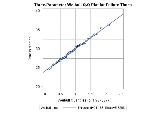
This example compares the use of three-parameter and two-parameter Weibull Q-Q plots for the failure times in months for 48 integrated circuits. The times are assumed to follow a Weibull distribution.
data Failures;
   input Time @@;
   label Time='Time in Months';
   datalines;
29.42 32.14 30.58 27.50 26.08 29.06 25.10 31.34
29.14 33.96 30.64 27.32 29.86 26.28 29.68 33.76
29.32 30.82 27.26 27.92 30.92 24.64 32.90 35.46
30.28 28.36 25.86 31.36 25.26 36.32 28.58 28.88
26.72 27.42 29.02 27.54 31.60 33.46 26.78 27.82
29.18 27.94 27.66 26.42 31.00 26.64 31.44 32.52
 ;
If no assumption is made about the parameters of this distribution, you can use the WEIBULL option to request a three-parameter Weibull plot. As in the previous example, you can visually estimate the shape parameter c by requesting plots for different values of c and choosing the value of c that linearizes the point pattern. Alternatively, you can request a maximum likelihood estimate for c, as illustrated in the following statements produce Weibull plots for c = 1, 2 and 3:
title 'Three-Parameter Weibull Q-Q Plot for Failure Times';
proc capability data=Failures noprint;
   qqplot Time / weibull(c=est theta=est sigma=est)
                 square
                 href=0.5 1 1.5 2
                 vref=25 27.5 30 32.5 35
                 odstitle=title;
run;
Note: When using the WEIBULL option, you must either specify a list of values for the Weibull shape parameter c with the C= option, or you must specify C=EST.
Output 5.23.1 displays the plot for the estimated value c = 1.99. The reference line corresponds to the estimated values for the threshold and scale parameters of (![]() =24.19 and
=24.19 and ![]() =5.83, respectively.
=5.83, respectively.
Note: See Creating Weibull Q-Q Plots in the SAS/QC Sample Library.
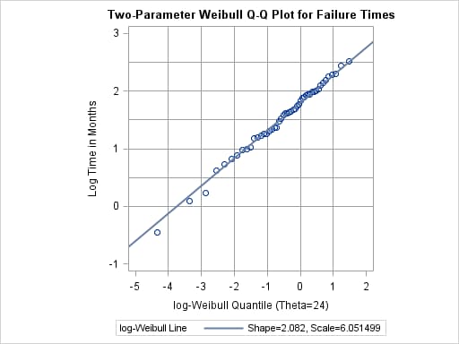
Now, suppose it is known that the circuit lifetime is at least 24 months. The following statements use the threshold value
![]() to produce the two-parameter Weibull Q-Q plot shown in Output 5.23.2:
to produce the two-parameter Weibull Q-Q plot shown in Output 5.23.2:
title 'Two-Parameter Weibull Q-Q Plot for Failure Times';
proc capability data=Failures noprint;
   qqplot Time / weibull2(theta=24 c=est sigma=est) square
                 href= -4 to 1
                 vref= 0 to 2.5 by 0.5
                 odstitle=title;
run;
The reference line is based on maximum likelihood estimates ![]() =2.08 and
=2.08 and ![]() =6.05. These estimates agree with those of the previous example.
=6.05. These estimates agree with those of the previous example.